Artificial intelligence and 3D subsurface interpretation for bright spot and channel detections

Yasir Bashir; Muhammad Afiq Aiman Bin Zahari; Abdullah Karaman; Doğa Doğan; Zeynep Döner; Ali Mohammadi; Syed Haroon Ali; Yasir Bashir; Muhammad Afiq Aiman Bin Zahari; Abdullah Karaman; Doğa Doğan; Zeynep Döner; Ali Mohammadi; Syed Haroon Ali

doi:10.3934/geosci.2024034

AIMS Geosciences

2024, Volume 10, Issue 4: 662-683. doi: 10.3934/geosci.2024034

Previous Article Next Article

Research article Topical Sections

Artificial intelligence and 3D subsurface interpretation for bright spot and channel detections

1.
Department of Geophysical Engineering, Faculty of Mines, İstanbul Technical University, İstanbul, Türkiye
2.
Faculty of Science, Universiti Teknologi Malaysia (UTM), Johor Bahru, Malaysia
3.
Department of Geological Engineering, Faculty of Mines, İstanbul Technical University, İstanbul, Türkiye
4.
Eurasia Institute of Earth Sciences, İstanbul Technical University, Istanbul, Türkiye
5.
Department of Earth Sciences, University of Sargodha, Sargodha, Punjab, Pakistan

Received: 31 May 2024 Revised: 29 July 2024 Accepted: 13 August 2024 Published: 04 September 2024

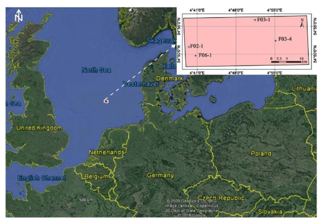
Seismic interpretation is primarily concerned with accurately characterizing underground geological structures & lithology and identifying hydrocarbon-containing rocks. The carbonates in the Netherlands have attracted considerable interest lately because of their potential as a petroleum or geothermal system. This is mainly because of the discovery of outstanding reservoir characteristics in the region. We employed global 3D seismic data and a novel Relative Geological Time (RGT) model using artificial intelligence (AI) to delve deeper into the analysis of the basin and petroleum resource reservoir. Several surface horizons were interpreted, each with a minimum spatial and temporal patch size, to obtain a comprehensive understanding of the subsurface. The horizons were combined with seismic attributes such as Root mean square (RMS) amplitude, spectral decomposition, and RGB Blending, enhancing the identification of the geological features in the field. The hydrocarbon potential of these sediments was mainly affected by the presence of a karst-related reservoir and migration pathways originating from a source rock of satisfactory quality. Our results demonstrated the importance of investigations on hydrocarbon potential and the development of 3D models. These findings enhance our understanding of the subsurface and oil systems in the area.

Keywords:

Citation: Yasir Bashir, Muhammad Afiq Aiman Bin Zahari, Abdullah Karaman, Doğa Doğan, Zeynep Döner, Ali Mohammadi, Syed Haroon Ali. Artificial intelligence and 3D subsurface interpretation for bright spot and channel detections[J]. AIMS Geosciences, 2024, 10(4): 662-683. doi: 10.3934/geosci.2024034

Related Papers:

[1]	Ahmed M.A. El-Sayed, Eman M.A. Hamdallah, Hameda M. A. Alama . Multiple solutions of a Sturm-Liouville boundary value problem of nonlinear differential inclusion with nonlocal integral conditions. AIMS Mathematics, 2022, 7(6): 11150-11164. doi: 10.3934/math.2022624
[2]	Murugesan Manigandan, Kannan Manikandan, Hasanen A. Hammad, Manuel De la Sen . Applying fixed point techniques to solve fractional differential inclusions under new boundary conditions. AIMS Mathematics, 2024, 9(6): 15505-15542. doi: 10.3934/math.2024750
[3]	Mouffak Benchohra, John R. Graef, Nassim Guerraiche, Samira Hamani . Nonlinear boundary value problems for fractional differential inclusions with Caputo-Hadamard derivatives on the half line. AIMS Mathematics, 2021, 6(6): 6278-6292. doi: 10.3934/math.2021368
[4]	Bashir Ahmad, Badrah Alghamdi, Ahmed Alsaedi, Sotiris K. Ntouyas . Existence results for Riemann-Liouville fractional integro-differential inclusions with fractional nonlocal integral boundary conditions. AIMS Mathematics, 2021, 6(7): 7093-7110. doi: 10.3934/math.2021416
[5]	Madeaha Alghanmi, Shahad Alqurayqiri . Existence results for a coupled system of nonlinear fractional functional differential equations with infinite delay and nonlocal integral boundary conditions. AIMS Mathematics, 2024, 9(6): 15040-15059. doi: 10.3934/math.2024729
[6]	Abdissalam Sarsenbi, Abdizhahan Sarsenbi . Boundary value problems for a second-order differential equation with involution in the second derivative and their solvability. AIMS Mathematics, 2023, 8(11): 26275-26289. doi: 10.3934/math.20231340
[7]	Adel Lachouri, Mohammed S. Abdo, Abdelouaheb Ardjouni, Bahaaeldin Abdalla, Thabet Abdeljawad . On a class of differential inclusions in the frame of generalized Hilfer fractional derivative. AIMS Mathematics, 2022, 7(3): 3477-3493. doi: 10.3934/math.2022193
[8]	Djamila Chergui, Taki Eddine Oussaeif, Merad Ahcene . Existence and uniqueness of solutions for nonlinear fractional differential equations depending on lower-order derivative with non-separated type integral boundary conditions. AIMS Mathematics, 2019, 4(1): 112-133. doi: 10.3934/Math.2019.1.112
[9]	Nayyar Mehmood, Niaz Ahmad . Existence results for fractional order boundary value problem with nonlocal non-separated type multi-point integral boundary conditions. AIMS Mathematics, 2020, 5(1): 385-398. doi: 10.3934/math.2020026
[10]	Najla Alghamdi, Bashir Ahmad, Esraa Abed Alharbi, Wafa Shammakh . Investigation of multi-term delay fractional differential equations with integro-multipoint boundary conditions. AIMS Mathematics, 2024, 9(5): 12964-12981. doi: 10.3934/math.2024632

Abstract

1. Introduction

The models of the differential and integral equations have been appeared in different applications (see ^{[1,2,3,4,6,7,9,12,13,14,15,16,17,18,19,20]}).

Boundary value problems involving fractional differential equations arise in physical sciences and applied mathematics. In some of these problems, subsidiary conditions are imposed locally. In some other cases, nonlocal conditions are imposed. It is sometimes better to impose nonlocal conditions since the measurements needed by a nonlocal condition may be more precise than the measurement given by a local condition. Consequently, a variety of excellent results on fractional boundary value problems (abbreviated BVPs) with resonant conditions have been achieved. For instance, Bai ^[4] studied a type of fractional differential equations with m-points boundary conditions. The existence of nontrivial solutions was established by using coincidence degree theory. Applying the same method, Kosmatov ^[17] investigated the fractional order three points BVP with resonant case.

Although the study of fractional BVPs at resonance has acquired fruitful achievements, it should be noted that such problems with Riemann-Stieltjes integrals are very scarce, so it is worthy of further explorations. Riemann-Stieltjes integral has been considered as both multipoint and integral in a single framework, which is more common, see the relevant works due to Ahmad et al. ^[1].

The boundary value problems with nonlocal, integral and infinite points boundary conditions have been studied by some authors (see, for example ^[8,10,11,12]).

Here, we discuss the boundary value problem of the nonlinear differential inclusions of arbitrary (fractional) orders

$\begin{equation} \frac{dx}{dt}\in F_{1}(t,x(t),I^{\gamma}f_{2}(t,D^{\alpha}x(t))),\; \; \alpha,\gamma\in(0,1] \; \; \; \; t\in(0,1) \end{equation}$

(1.1)

with the nonlocal boundary condition

$\begin{equation} {{\sum\limits^{m}_{k = 1} a_{k}}} x(\tau_{k} ) = x_{0},\; a_{k} > 0\; \; \tau_{k}\in[0,1], \end{equation}$

(1.2)

the integral condition

$\begin{equation} \int_{0}^{1}x(s)dg(s) = x_{0} \end{equation}$

(1.3)

and the infinite point boundary condition

$\begin{equation} {{\sum\limits^{\infty}_{k = 1} a_{k}}} x(\tau_{k} ) = x_{0},\; a_{k} > 0\; and\; \tau_{k}\in[0,1]. \end{equation}$

(1.4)

We study the existence of solutions $x\in C[0, 1]$ of the problems (1.1) and (1.2), and deduce the existence of solutions of the problem of (1.1) with the conditions (1.3) and (1.4). Then the existence of the maximal and minimal solutions will be proved. The sufficient condition for the uniqueness and continuous dependence of the solution will be studied.

This paper is organised as: In Section 2, we prove the existence of continuous solutions of the problems (1.1) and (1.2), and deduce the existence of solutions of the problem of (1.1) with the conditions (1.3) and (1.4). In Section 3, the existence of the maximal and minimal solutions is proved. In Section 4, the sufficient condition for the uniqueness and continuous dependence of the solution are studied. Next, in Section 5, we extend our results to the nonlocal problems (1.3) and (2.1). Finally, some existence results is proved for the nonlocal problems (1.4) and (2.1) in Section 6.

2. Main results

Consider the following assumptions:

(I) (i) The set $F_{1}(t, x, y)$ is nonempty, closed and convex for all $(t, x, y)\in [0, 1]\times R\times R$ .

(ii) $F_{1}(t, x, y)$ is measurable in $t\in [0, 1]$ for every $x, y\in R$ .

(iii) $F_{1}(t, x, y)$ is upper semicontinuous in $x$ and $y$ for every $t\in [0, 1]$ .

(iv) There exist a bounded measurable function $a_{1}: [0, 1]\longrightarrow R$ and a positive constant $K_{1}$ , such that

$\begin{eqnarray*} \|F_{1}(t,x,y)\|& = &\sup\{|f_{1}|:f_{1}\in F_{1}(t,x,y)\}\\ &\leq& |a_{1}(t)|+K_{1}(|x|+|y|). \end{eqnarray*}$

Remark 2.1. From the assumptions (i)–(iv) we can deduce that (see ^[3,6,7,13]) there exists $f_{1}\in F_{1}(t, x, y)$ , such that

(v) $f_{1}:[0, 1]\times R\times R\longrightarrow R$ is measurable in $t$ for every $x, y\in R$ and continuous in $x, y$ for $t\in [0, 1]$ , and there exist a bounded measurable function $a_{1}:[0, 1]\rightarrow R$ and a positive constant $K_{1} > 0$ such that

$|f_{1}(t,x,y)|\leq |a_{1}(t)|+K_{1}(|x|+|y|),$

and the functional $f_{1}$ satisfies the differential equation

$\begin{equation} \frac{dx}{dt} = f_{1}(t,x(t),I^{\gamma}f_{2}(t,D^{\alpha}x(t))),\; \; \alpha,\gamma\in(0,1]\; and\; t\in(0,1]. \end{equation}$

(2.1)

(II) $f_{2}:[0, 1]\times R\longrightarrow R$ is measurable in $t$ for any $x\in R$ and continuous in $x$ for $t\in [0, 1]$ , and there exist a bounded measurable function $a_{2}:[0, 1]\rightarrow R$ and a positive constant $K_{2} > 0$ such that

$|f_{2}(t,x)|\leq |a_{2}(t)|+K_{2}|x|,\; \forall t\in [0,1]\; \; \mbox {and}\; x\in R$

and

$\sup\limits_{t\in [0,1]}|a_{i}(t)|\leq a_{i}, i = 1,2.$

(III) $2K_{1}\gamma+K_{1}K_{2}\alpha < \alpha\gamma\Gamma(2-\alpha), \; \alpha, \gamma \in (0, 1].$

Remark 2.2. From (I) and (v) we can deduce that every solution of (1.1) is a solution of (2.1). Now, we shall prove the following lemma.

Lemma 2.1. If the solution of the problems (1.2)–(2.1) exists then it can be expressed by the integral equation

$\begin{eqnarray} y(t)& = &\int_{0}^{t}\frac{(t-s)^{-\alpha}}{\Gamma(1-\alpha)} f_{1}(s,\frac{1}{\sum\limits^{m}_{k = 1}a_{k}}[x_{0}-\sum\limits^{m}_{k = 1}a_{k}\int_{0}^{\tau_{k}}\frac{(\tau_{k}-\theta)^{\alpha-1}} {\Gamma(\alpha)}y(\theta)d\theta]\\ &&+\int_{0}^{s}\frac{(s-\theta)^{\alpha-1}}{\Gamma(\alpha)}y(\theta)d\theta,\int_{0}^{s}\frac{(s-\theta)^{\gamma-1}} {\Gamma(\gamma)}f_{2}(\phi,y(\theta))d\theta)ds. \end{eqnarray}$

(2.2)

Proof. Consider the boundary value problems (1.2)–(2.1) be satisfied. Operating by $I^{1-\alpha}$ on both sides of (2.1) we can obtain

$\begin{equation} D^{\alpha}x(t) = I^{1-\alpha}\frac{dx}{dt} = I^{1-\alpha} f_{1}(t,x(t),I^{\gamma}f_{2}(t,D^{\alpha}x(t))). \end{equation}$

(2.3)

Taking

$\begin{equation} D^{\alpha}x(t) = y(t), \end{equation}$

(2.4)

then we obtain

$\begin{equation} x(t) = x(0)+I^{\alpha}y(t). \end{equation}$

(2.5)

Putting $t = \tau$ and multiplying (2.5) by $\Sigma_{k = 1}^{m}a_{k}$ , then we get

$\begin{equation} \Sigma_{k = 1}^{m}a_{k}x(\tau_{k}) = \Sigma_{k = 1}^{m}a_{k}x(0)+\Sigma_{k = 1}^{m}a_{k}I^{\alpha}y(\tau_{k}), \end{equation}$

(2.6)

$\begin{equation} x_{0} = \Sigma_{k = 1}^{m}a_{k}x(0)+\Sigma_{k = 1}^{m}a_{k}I^{\alpha}y(\tau_{k}) \end{equation}$

(2.7)

and

$\begin{equation} x(0) = \frac{1}{\Sigma_{k = 1}^{m}a_{k}}[x_{0}-\Sigma_{k = 1}^{m}a_{k}I^{\alpha}y(\tau_{k})]. \end{equation}$

(2.8)

Then

$\begin{equation} x(t) = \frac{1}{\Sigma_{k = 1}^{m}a_{k}}[x_{0}-\Sigma_{k = 1}^{m}a_{k}I^{\alpha}y(\tau_{k})]+I^{\alpha}y(t). \end{equation}$

(2.9)

Substituting (2.8) and (2.9) in (2.5), which completes the proof.

Theorem 2.1. Let assumptions (I)–(III) be satisfied. Then the integral equation (2.2) has at least one continuous solution.

Proof. Define a set $Q_{r}$ as

$Q_{r} = \{y\in C[0,1]:\|y\|\leq r\},\; \;$

$\begin{eqnarray*} r = \frac{\Gamma(\gamma+1)[a_{1}+K_{1}A|x_{0}|]+k_{1}a_{2}}{\alpha\gamma\Gamma(2-\alpha)-[2K_{1}\alpha+K_{1}K_{2}\gamma]},\; \; \; (\sum\limits^{m}_{k = 1}a_{k})^{-1} = A, \end{eqnarray*}$

and the operator $F$ by

$\begin{eqnarray*} Fy(t)& = &\int_{0}^{t}\frac{(t-s)^{-\alpha}}{\Gamma(1-\alpha)} f_{1}(s,\frac{1}{\sum\limits^{m}_{k = 1}a_{k}}[x_{0}-\sum\limits^{m}_{k = 1}a_{k}\int_{0}^{\tau_{k}}\frac{(\tau_{k}-\theta)^{\alpha-1}}{\Gamma(\alpha)}y(\theta)d\theta]\\ &&+\int_{0}^{s}\frac{(s-\theta)^{\alpha-1}}{\Gamma(\alpha)}y(\theta)d\theta,\int_{0}^{s}\frac{(s-\theta)^{\gamma-1}}{\Gamma(\gamma)}f_{2}(\theta,y(\theta))d\theta)ds. \end{eqnarray*}$

For $y\in Q_{r}$ , then

$\begin{eqnarray*} |Fy(t)|& = &|\int_{0}^{t}\frac{(t-s)^{-\alpha}}{\Gamma(1-\alpha)} f_{1}(s,\frac{1}{\sum\limits^{m}_{k = 1}a_{k}}[x_{0}-\sum\limits^{m}_{k = 1}a_{k}\int_{0}^{\tau_{k}}\frac{(\tau_{k}-\theta)^{\alpha-1}} {\Gamma(\alpha)}y(\theta)d\theta]\\ &&+\int_{0}^{s}\frac{(s-\theta)^{\alpha-1}}{\Gamma(\alpha)}y(\theta)d\theta,\int_{0}^{s}\frac{(s-\theta)^{\gamma-1}} {\Gamma(\gamma)}f_{2}(\theta,y(\theta))d\theta)ds|\\ &\leq& K_{1}\int_{0}^{t}\frac{(t-s)^{-\alpha}}{\Gamma(1-\alpha)}[\frac{|x_{0}|}{\sum\limits^{m}_{k = 1}a_{k}}+\frac{\sum\limits^{m}_{k = 1} a_{k}\int_{0}^{\tau_{k}}\frac{(\tau_{k}-\theta)^{\alpha-1}}{\Gamma(\alpha)}|y(\theta)|d\theta}{\sum\limits^{m}_{k = 1}a_{k}}\\ &&+\int_{0}^{s}\frac{(s-\theta)^{\alpha-1}}{\Gamma(\alpha)}|y(\theta)|d\theta+\int_{0}^{s}\frac{(s-\phi)^{\gamma-1}} {\Gamma(\gamma)}(K_{2}|y(\theta)|+|a_{2}(t)|)d\theta]+|a_{1}(t)|)ds\\ &\leq& \frac{1}{\Gamma(2-\alpha)}[K_{1}A|x_{0}|+\frac{K_{1}\|y\|}{\Gamma(\alpha+1)}+K_{1}\frac{\|y\|}{\Gamma(\alpha+1)} +\frac{K_{1}K_{2}\|y\|}{\Gamma(\gamma+1)}+\frac{K_{1}a_{2}}{\Gamma(\gamma+1)}+a_{1}]\\ &\leq& \frac{1}{\Gamma(2-\alpha)}[K_{1}A|x_{0}|+\frac{K_{1}r}{\Gamma(\alpha+1)}+K_{1}\frac{r}{\Gamma(\alpha+1)}+ \frac{K_{1}K_{2}r}{\Gamma(\gamma+1)}+\frac{K_{1}a_{2}}{\Gamma(\gamma+1)}+a_{1}]\\ &\leq& \frac{1}{\Gamma(2-\alpha)}[K_{1}A|x_{0}|+\frac{2K_{1}r}{\Gamma(\alpha+1)}+\frac{K_{1}K_{2}r}{\Gamma(\gamma+1)}+ \frac{K_{1}a_{2}}{\Gamma(\gamma+1)}+a_{1}]\; \leq r. \end{eqnarray*}$

Thus, the class of functions $\{Fy\}$ is uniformly bounded on $Q_{r}$ and $F:Q_{r}\rightarrow Q_{r}$ . Let $y\in Q_{r}$ and $t_{1}, t_{2}\in [0, 1]$ such that $|t_{2}-t_{1}| < \delta$ , then

$\begin{eqnarray*} &&|Fy(t_{2})-Fy(t_{1})|\\ & = &|\int_{0}^{t_{2}}\frac{(t_{2}-s)^{-\alpha}}{\Gamma(1-\alpha)} (f_{1}(s,x(s),I^{\gamma}f_{2}(s,y(s)))ds-\int_{0}^{t_{1}}\frac{(t_{1}-s)^{-\alpha}}{\Gamma(1-\alpha)} (f_{1}(s,x(s),I^{\gamma}f_{2}(s,y(s)))ds|\\ &\leq&|\int_{0}^{t_{2}}\frac{(t_{2}-s)^{-\alpha}}{\Gamma(1-\alpha)} (f_{1}(s,x(s),I^{\gamma}f_{2}(s,y(s)))ds-\int_{0}^{t_{1}}\frac{(t_{2}-s)^{-\alpha}}{\Gamma(1-\alpha)} (f_{1}(s,x(s),I^{\gamma}f_{2}(s,y(s)))ds\\ &&+\int_{0}^{t_{1}}\frac{(t_{2}-s)^{-\alpha}}{\Gamma(1-\alpha)} (f_{1}(s,x(s),I^{\gamma}f_{2}(s,y(s)))ds-\int_{0}^{t_{1}}\frac{(t_{1}-s)^{-\alpha}}{\Gamma(1-\alpha)} (f_{1}(s,x(s),I^{\gamma}f_{2}(s,y(s)))ds|\\ &\leq&\int_{t_{1}}^{t_{2}}\frac{(t_{2}-s)^{-\alpha}}{\Gamma(1-\alpha)} |(f_{1}(s,x(s),I^{\gamma}f_{2}(s,y(s)))|ds\\ &&+\int_{0}^{t_{1}}\frac{(t_{2}-s)^{-\alpha}-(t_{1}-s)^{-\alpha}}{\Gamma(1-\alpha)} |(f_{1}(s,x(s),I^{\gamma}f_{2}(s,y(s)))ds|\\ &\leq&\int_{t_{1}}^{t_{2}}\frac{(t_{2}-s)^{-\alpha}}{\Gamma(1-\alpha)} |(f_{1}(s,x(s),I^{\gamma}f_{2}(s,y(s)))|ds\\ &&+\int_{0}^{t_{1}}\frac{(t_{2}-s)^{\alpha}-(t_{1}-s)^{\alpha}}{\Gamma(1-\alpha)(t_{2}-s)^{\alpha}(t_{1}-s)^{\alpha}}. |(f_{1}(s,x(s),I^{\gamma}f_{2}(s,y(s)))|ds. \end{eqnarray*}$

Thus, the class of functions $\{Fy\}$ is equicontinuous on $Q_{r}$ and $\{Fy\}$ is compact operator by the Arzela-Ascoli Theorem ^[5].

Now we prove that $F$ is continuous operator. Let ${y_{n}}\subset Q_{r}$ be convergent sequence such that $y_{n}\rightarrow y$ , then

$\begin{eqnarray*} Fy_{n}(t)& = &\int_{0}^{t}\frac{(t-s)^{-\alpha}}{\Gamma(1-\alpha)} f_{1}(s,\frac{1}{\sum\nolimits^{m}_{k = 1}a_{k}}[x_{0}-\sum\limits^{m}_{k = 1}a_{k}\int_{0}^{\tau_{k}}\frac{(\tau_{k}-\theta)^{\alpha-1}}{\Gamma(\alpha)}y_{n}(\theta)d\theta]\\ &&+\int_{0}^{s}\frac{(s-\theta)^{\alpha-1}}{\Gamma(\alpha)}y_{n}(\theta)d\theta, \int_{0}^{s}\frac{(s-\theta)^{\gamma-1}}{\Gamma(\gamma)}f_{2}(\theta,y_{n}(\theta)))ds. \end{eqnarray*}$

Using Lebesgue dominated convergence Theorem ^[5] and assumptions (iv)–(II) we have

$\begin{eqnarray*} \lim\limits_{n\to \infty} Fy_{n}(t)& = &\lim\limits_{n\to \infty}\int_{0}^{t}\frac{(t-s)^{-\alpha}}{\Gamma(1-\alpha)} f_{1}(s,\frac{1}{\sum\nolimits^{m}_{k = 1}a_{k}}[x_{0}-\sum\limits^{m}_{k = 1}a_{k}\int_{0}^{\tau_{k}}\frac{(\tau_{k}-\theta)^{\alpha-1}}{\Gamma(\alpha)}y_{n}(\theta)d\theta]\\ &&+\int_{0}^{s}\frac{(s-\theta)^{\alpha-1}}{\Gamma(\alpha)}y_{n}(\theta)d\theta,\int_{0}^{s}\frac{(s-\theta)^{\gamma-1}}{\Gamma(\gamma)}f_{2}(\theta,y_{n}(\theta)))ds\\ & = &\int_{0}^{t}\frac{(t-s)^{-\alpha}}{\Gamma(1-\alpha)} f_{1}(s,\frac{1}{\sum\nolimits^{m}_{k = 1}a_{k}}[x_{0}-\sum\limits^{m}_{k = 1}a_{k}\int_{0}^{\tau_{k}}\frac{(\tau_{k}-\theta)^{\alpha-1}}{\Gamma(\alpha)}\lim\limits_{n\to \infty}y_{n}(\theta)d\theta]\\ &&+\int_{0}^{s}\frac{(s-\theta)^{\alpha-1}}{\Gamma(\alpha)}\lim\limits_{n\to \infty}y_{n}(\theta)d\theta,\int_{0}^{s}\frac{(s-\theta)^{\gamma-1}}{\Gamma(\gamma)}f_{2}(\theta,\lim\limits_{n\to \infty}y_{n}(\theta)))ds\\ & = &\int_{0}^{t}\frac{(t-s)^{-\alpha}}{\Gamma(1-\alpha)} f_{1}(s,\frac{1}{\sum\nolimits^{m}_{k = 1}a_{k}}[x_{0}-\sum\limits^{m}_{k = 1}a_{k}\int_{0}^{\tau_{k}}\frac{(\tau_{k}-\theta)^{\alpha-1}}{\Gamma(\alpha)}y(\theta)d\theta]\\ &&+\int_{0}^{s}\frac{(s-\theta)^{\alpha-1}}{\Gamma(\alpha)}y(\theta)d\theta,\int_{0}^{s}\frac{(s-\theta)^{\gamma-1}}{\Gamma(\gamma)}f_{2} (\theta,y(\theta)))ds\; = \; Fy(t). \end{eqnarray*}$

Then $F:Q_{r}\rightarrow Q_{r}$ is continuous, and by Schauder Fixed Point Theorem^[5] there exists at least one solution $y\in C[0, 1]$ of (2.2). Now

$\begin{eqnarray*} \frac{dx}{dt}& = &\frac{d}{dt}[x(0)+I^{\alpha}y(t)]\\ & = &\frac{d}{dt}I^{\alpha}I^{1-\alpha}f_{1}(t,x(t),I^{\gamma}f_{2}(t,y(t)))\\ & = &\frac{d}{dt}If_{1}(t,x(t),I^{\gamma}f_{2}(t,y(t)))\\ & = &f_{1}(t,x(t),I^{\gamma}f_{2}(t,y(t))). \end{eqnarray*}$

Putting $t = \tau$ and using (2.9), we obtain

$\begin{eqnarray*} &&x(t) = \frac{1}{\Sigma_{k = 1}^{m}a_{k}}[x_{0}-\Sigma_{k = 1}^{m}a_{k}I^{\alpha}y(\tau_{k})]+I^{\alpha}y(t),\\ &&\Sigma_{k = 1}^{m}a_{k}x(\tau_{k}) = \Sigma_{k = 1}^{m}a_{k}\frac{1}{\Sigma_{k = 1}^{m}a_{k}}[x_{0}-\Sigma_{k = 1}^{m}a_{k}I^{\alpha}y(\tau_{k})]+\Sigma_{k = 1}^{m}a_{k}I^{\alpha}y(\tau_{k}), \end{eqnarray*}$

then

$\begin{eqnarray*} &&\Sigma_{k = 1}^{m}a_{k}x(\tau_{k}) = x_{0}, \; a_{k} > 0\; and\; \tau_{k}\in[0,1]. \end{eqnarray*}$

This proves the equivalence between the problems (1.2)–(2.1) and the integral equation (2.2). Then there exists at least one solution $y\in C[0, 1]$ of the problems (1.2)–(2.1).

3. Maximal and minimal solutions

Here, we shall study the maximal and minimal solutions for the problems (1.2) and (2.1). Let $y(t)$ be any solution of (2.2), let $u(t)$ be a solution of (2.2), then $u(t)$ is said to be a maximal solution of (2.2) if it satisfies the inequality

$y(t)\leq u(t),\; \; \; t\in[0,1].$

A minimal solution can be defined by similar way by reversing the above inequality.

Lemma 3.1. Let the assumptions of Theorem 2.1 be satisfied. Assume that $x(t)$ and $y(t)$ are two continuous functions on $[0, 1]$ satisfying

$\begin{eqnarray*} y(t)&\leq&\int_{0}^{t}\frac{(t-s)^{-\alpha}}{\Gamma(1-\alpha)} f_{1}(s,\frac{1}{\sum\nolimits^{m}_{k = 1}a_{k}}[x_{0}-\sum\limits^{m}_{k = 1}a_{k}\int_{0}^{\tau_{k}}\frac{(\tau_{k}-\theta)^{\alpha-1}}{\Gamma(\alpha)}y(\theta)d\theta]\\ &&+\int_{0}^{s}\frac{(s-\theta)^{\alpha-1}}{\Gamma(\alpha)}y(\theta)d\theta,\int_{0}^{s}\frac{(s-\theta)^{\gamma-1}}{\Gamma(\gamma)}f_{2}(\theta,y(\theta)))ds\; \; t\in[0,1],\\ x(t)&\geq&\int_{0}^{t}\frac{(t-s)^{-\alpha}}{\Gamma(1-\alpha)} f_{1}(s,\frac{1}{\sum\nolimits^{m}_{k = 1}a_{k}}[x_{0}-\sum\limits^{m}_{k = 1}a_{k}\int_{0}^{\tau_{k}}\frac{(\tau_{k}-\theta)^{\alpha-1}}{\Gamma(\alpha)}x(\theta)d\theta]\\ &&+\int_{0}^{s}\frac{(s-\theta)^{\alpha-1}}{\Gamma(\alpha)}x(\theta)d\theta,\int_{0}^{s}\frac{(s-\theta)^{\gamma-1}}{\Gamma(\gamma)}f_{2} (\theta,x(\theta)))ds\; \; t\in[0,1], \end{eqnarray*}$

where one of them is strict.

Let functions $f_{1}$ and $f_{2}$ be monotonic nondecreasing in $y$ , then

$\begin{equation} y(t) < x(t),\; \; \; t > 0. \end{equation}$

(3.1)

Proof. Let the conclusion (3.1) be not true, then there exists $t_{1}$ with

$y(t_{1}) < x(t_{1}),\; \; \; t_{1} > 0\; \; \; \mbox{and}\; \; \; y(t) < x(t),\; \; \; 0 < t < t_{1}.$

Since $f_{1}$ and $f_{2}$ are monotonic functions in $y,$ then we have

$\begin{eqnarray*} y(t_{1})&\leq&\int_{0}^{t_{1}}\frac{(t_{1}-s)^{-\alpha}}{\Gamma(1-\alpha)} f_{1}(s,\frac{1}{\sum\nolimits^{m}_{k = 1}a_{k}}[x_{0}-\sum\limits^{m}_{k = 1}a_{k}\int_{0}^{\tau_{k}}\frac{(\tau_{k}-\theta)^{\alpha-1}}{\Gamma(\alpha)}y(\theta)d\theta]\\ &&+\int_{0}^{s}\frac{(s-\theta)^{\alpha-1}}{\Gamma(\alpha)}y(\theta)d\theta,\int_{0}^{s}\frac{(s-\theta)^{\gamma-1}}{\Gamma(\gamma)}f_{2}(\theta,y(\theta)))ds\\ & < &\int_{0}^{t_{1}}\frac{(t-s)^{-\alpha}}{\Gamma(1-\alpha)} f_{1}(s,\frac{1}{\sum\nolimits^{m}_{k = 1}a_{k}}[x_{0}-\sum\limits^{m}_{k = 1}a_{k}\int_{0}^{\tau_{k}}\frac{(\tau_{k}-\theta)^{\alpha-1}}{\Gamma(\alpha)}x(\theta)d\theta]\\ &&+\int_{0}^{s}\frac{(s-\theta)^{\alpha-1}}{\Gamma(\alpha)}x(\theta)d\theta,\int_{0}^{s}\frac{(s-\theta)^{\gamma-1}}{\Gamma(\gamma)}f_{2} (\theta,x(\theta)))ds\\ & < &x(t_{1}),\; t_{1}\in[0,1]. \end{eqnarray*}$

This contradicts the fact that $y(t_{1}) = x(t_{1})$ , then $y(t) < x(t)$ . This completes the proof.

For the existence of the continuous maximal and minimal solutions for (2.1), we have the following theorem.

Theorem 3.1. Let the assumptions of Theorem 2.1 be hold. Moreover, if $f_{1}$ and $f_{2}$ are monotonic nondecreasing functions in $y$ for each $t\in [0, 1]$ , then Eq (2.1) has maximal and minimal solutions.

Proof. First, we should demonstrate the existence of the maximal solution of (2.1). Let $\epsilon > 0$ be given. Now consider the integral equation

$\begin{eqnarray} y_{\epsilon}(t)& = &\int_{0}^{t}\frac{(t-s)^{-\alpha}}{\Gamma(1-\alpha)} f_{1,\epsilon}\bigg(s,\frac{1}{\sum\nolimits^{m}_{k = 1}a_{k}}[x_{0}-\sum\limits^{m}_{k = 1}a_{k}\int_{0}^{\tau_{k}}\frac{(\tau_{k}-\theta)^{\alpha-1}} {\Gamma(\alpha)}y_{\epsilon}(\theta)d\theta]\\ &&+\int_{0}^{s}\frac{(s-\theta)^{\alpha-1}}{\Gamma(\alpha)}y_\epsilon(\theta)d\theta,\int_{0}^{s} \frac{(s-\theta)^{\gamma-1}}{\Gamma(\gamma)}f_{2,\epsilon}(\theta,y_{\epsilon}(\theta))d\theta \bigg)ds,\; \; t\in[0,1], \end{eqnarray}$

where

$f_{1,\epsilon}(s,x_{\epsilon}(s),y_{\epsilon}(s) ) = f_{1}(s,x_{\epsilon}(s),y_{\epsilon}(s))+\epsilon,$

$f_{2,\epsilon}(s,x_{\epsilon}(s)) = f_{2}(s,x_{\epsilon}(s))+\epsilon.$

For $\epsilon_{2} > \epsilon_{1},$ we have

$\begin{eqnarray} y_{\epsilon_{2}}(t)& = &\int_{0}^{t}\frac{(t-s)^{-\alpha}}{\Gamma(1-\alpha)} f_{1,\epsilon_2}\bigg(s,\frac{1}{\sum\nolimits^{m}_{k = 1}a_{k}}[x_{0}-\sum\limits^{m}_{k = 1}a_{k}\int_{0}^{\tau_{k}}\frac{(\tau_{k}-\theta)^{\alpha-1}}{\Gamma(\alpha)}y_{\epsilon_{2}}(\theta)d\theta]\\ &&+\int_{0}^{s}\frac{(s-\theta)^{\alpha-1}}{\Gamma(\alpha)}y_{\epsilon_{2}}(\theta)d\theta,\int_{0}^{s} \frac{(s-\theta)^{\gamma-1}}{\Gamma(\gamma)}f_{2,\epsilon_{2}}(\theta,y_{\epsilon_{2}}(\theta))d\theta\bigg )ds,\; \; t\in[0,1], \end{eqnarray}$

$\begin{eqnarray} y_{\epsilon_{2}}(t)& = &\int_{0}^{t}\frac{(t-s)^{-\alpha}}{\Gamma(1-\alpha)} \bigg[f_{1}\bigg(s,\frac{1}{\sum\nolimits^{m}_{k = 1}a_{k}}[x_{0}-\sum\limits^{m}_{k = 1}a_{k}\int_{0}^{\tau_{k}}\frac{(\tau_{k}-\theta)^{\alpha-1}}{\Gamma(\alpha)}y_{\epsilon_{2}}(\theta)d\theta]\\ &&+\int_{0}^{s}\frac{(s-\theta)^{\alpha-1}}{\Gamma(\alpha)}y_{\epsilon_{2}}(\theta)d\theta,\int_{0}^{s} \frac{(s-\theta)^{\gamma-1}}{\Gamma(\gamma)}(f_{2}(\theta,y_{\epsilon_{2}}(\theta))+\epsilon_{2})d\theta \bigg)+\epsilon_2\bigg]ds,\; t\in[0,1]. \end{eqnarray}$

Also

$\begin{eqnarray*} y_{\epsilon_{1}}(t)& = &\int_{0}^{t}\frac{(t-s)^{-\alpha}}{\Gamma(1-\alpha)} f_{1,\epsilon_1}\bigg(s,\frac{1}{\sum\nolimits^{m}_{k = 1}a_{k}}[x_{0}-\sum\limits^{m}_{k = 1}a_{k}\int_{0}^{\tau_{k}}\frac{(\tau_{k}-\theta)^{\alpha-1}}{\Gamma(\alpha)}y_{\epsilon_{1}}(\theta)d\theta]\\ &&+\int_{0}^{s}\frac{(s-\theta)^{\alpha-1}}{\Gamma(\alpha)}y_{\epsilon_{1}}(\theta)d\theta,\int_{0}^{s}\frac{(s-\theta)^ {\gamma-1}}{\Gamma(\gamma)}f_{2,\epsilon_{1}}(\theta,y_{\epsilon_{1}}(\theta))d\theta\bigg)ds,\\ y_{\epsilon_{1}}(t)& = &\int_{0}^{t}\frac{(t-s)^{-\alpha}}{\Gamma(1-\alpha)} \bigg[f_{1}\bigg(s,\frac{1}{\sum\nolimits^{m}_{k = 1}a_{k}}[x_{0}-\sum\limits^{m}_{k = 1}a_{k}\int_{0}^{\tau_{k}}\frac{(\tau_{k}-\phi)^{\alpha-1}} {\Gamma(\alpha)}y_{\epsilon_{1}}(\theta)d\theta]\\ &&+\int_{0}^{s}\frac{(s-\theta)^{\alpha-1}}{\Gamma(\alpha)}y_{\epsilon_{1}}(\theta)d\theta,\int_{0}^{s} \frac{(s-\theta)^{\gamma-1}}{\Gamma(\gamma)}(f_{2}(\theta,y_{\epsilon_{1}}(\theta))+\epsilon_{1})d\theta \bigg)+\epsilon_1\bigg] ds \\ & > &\int_{0}^{t}\frac{(t-s)^{-\alpha}}{\Gamma(1-\alpha)} \bigg[f_{1}\bigg(s,\frac{1}{\sum\nolimits^{m}_{k = 1}a_{k}}[x_{0}-\sum\limits^{m}_{k = 1}a_{k}\int_{0}^{\tau_{k}}\frac{(\tau_{k}-\theta)^{\alpha-1}} {\Gamma(\alpha)}y_{\epsilon_{2}}(\theta)d\theta]\\ &&+\int_{0}^{s}\frac{(s-\theta)^{\alpha-1}}{\Gamma(\alpha)}y_{\epsilon_{2}}(\theta)d\theta,\int_{0}^{s} \frac{(s-\theta)^{\gamma-1}}{\Gamma(\gamma)}(f_{2}(\theta,y_{\epsilon_{2}}(\tau))+\epsilon_{2})d\theta \bigg)+\epsilon_2\bigg]ds. \end{eqnarray*}$

Applying Lemma 3.1, we obtain

$y_{\epsilon_{2}} < y_{\epsilon_{1}},\; t\in[0,1].$

As shown before, the family of function $y_{\epsilon}(t)$ is equi-continuous and uniformly bounded, then by Arzela Theorem, there exist decreasing sequence $\epsilon_{n}$ , such that $\epsilon_{n}\rightarrow 0$ as $n\rightarrow \infty$ , and $u(t) = {\lim_{n\rightarrow \infty}}y_{\epsilon_{n}}(t)$ exists uniformly in $[0, 1]$ and denote this limit by $u(t)$ . From the continuity of the functions, $f_{2, \epsilon_n}(t, y_{\epsilon_n}(t))$ , we get $f_{2, \epsilon_n}(t, y_{\epsilon_n}(t))\longrightarrow f_{2}(t, y(t))$ as $n\rightarrow \infty$ and

$\begin{eqnarray*} &&u(t) = \lim\limits_{n\rightarrow \infty}y_{\epsilon_{n}}(t) = \int_{0}^{t}\frac{(t-s)^{-\alpha}}{\Gamma(1-\alpha)} \bigg[f_{1}\bigg(s,\frac{1}{\sum\nolimits^{m}_{k = 1}a_{k}}[x_{0}-\sum\limits^{m}_{k = 1}a_{k}\int_{0}^{\tau_{k}}\frac{(\tau_{k}-\theta)^{\alpha-1}}{\Gamma(\alpha)}y_{\epsilon_{n}}(\theta)d\theta]\\ &&+\int_{0}^{s}\frac{(s-\theta)^{\alpha-1}}{\Gamma(\alpha)}y_{\epsilon_{n}}(\theta)d\theta, \int_{0}^{s}\frac{(s-\theta)^{\gamma-1}}{\Gamma(\gamma)}(f_{2}(\theta,y_{\epsilon_{n}}(\theta))+\epsilon_{n})\bigg)+\epsilon_n \bigg]ds,\; \; t\in[0,1]. \end{eqnarray*}$

Now we prove that $u(t)$ is the maximal solution of (2.1). To do this, let $y(t)$ be any solution of (2.1), then

$\begin{eqnarray*} y(t)& = &\int_{0}^{t}\frac{(t-s)^{-\alpha}}{\Gamma(1-\alpha)} f_{1}\bigg(s,\frac{1}{\sum\nolimits^{m}_{k = 1}a_{k}}[x_{0}-\sum\limits^{m}_{k = 1}a_{k}\int_{0}^{\tau_{k}}\frac{(\tau_{k}-\theta)^{\alpha-1}}{\Gamma(\alpha)}y(\theta)d\theta]\\ &&+\int_{0}^{s}\frac{(s-\theta)^{\alpha-1}}{\Gamma(\alpha)}y(\theta)d\theta,\int_{0}^{s}\frac{(s-\theta)^{\gamma-1}}{\Gamma(\gamma)}f_{2}(\theta,y(\theta))d\theta \bigg)ds,\\ y_{\epsilon}(t)& = &\int_{0}^{t}\frac{(t-s)^{-\alpha}}{\Gamma(1-\alpha)} \bigg[f_{1}\bigg(s,\frac{1}{\sum\nolimits^{m}_{k = 1}a_{k}}[x_{0}-\sum\limits^{m}_{k = 1}a_{k}\int_{0}^{\tau_{k}}\frac{(\tau_{k}-\theta)^{\alpha-1}}{\Gamma(\alpha)} y_{\epsilon}(\theta)d\theta]\\ &&+\int_{0}^{s}\frac{(s-\theta)^{\alpha-1}}{\Gamma(\alpha)}y_{\epsilon}(\theta)d\theta,\int_{0}^{s}\frac{(s-\theta)^{\gamma-1}}{\Gamma(\gamma)}(f_{2} (\theta,y_{\epsilon}(\theta))+\epsilon)d\theta \bigg)+\epsilon \bigg]ds \end{eqnarray*}$

and

$\begin{eqnarray*} y_{\epsilon}(t)& > &\int_{0}^{t}\frac{(t-s)^{-\alpha}}{\Gamma(1-\alpha)} f_{1}\bigg(s,\frac{1}{\sum\nolimits^{m}_{k = 1}a_{k}}[x_{0}-\sum\limits^{m}_{k = 1}a_{k}\int_{0}^{\tau_{k}}\frac{(\tau_{k}-\theta)^{\alpha-1}}{\Gamma(\alpha)}y_{\epsilon}(\theta)d\theta]\\ &&+\int_{0}^{s}\frac{(s-\theta)^{\alpha-1}}{\Gamma(\alpha)}y_{\epsilon}(\theta)d\theta,\int_{0}^{s}\frac{(s-\theta)^{\gamma-1}}{\Gamma(\gamma)} f_{2}(\theta,y_{\epsilon}(\theta))\bigg)ds. \end{eqnarray*}$

Applying Lemma 3.1, we obtain

$y(t) < y_{\epsilon}(t), t\in [0,1].$

From the uniqueness of the maximal solution it clear that $y_{\epsilon}(t)$ tends to $u(t)$ uniformly in $[0, 1]$ as $\epsilon\rightarrow 0.$

By a similar way as done above, we can prove the existence of the minimal solution.

4. Uniqueness of the solution

Here, we study the sufficient condition for the uniqueness of the solution $y\in C[0, 1]$ of problems (1.2) and (2.1). Consider the following assumptions:

( $I^{*}$ ) (i) The set $F_{1}(t, x, y)$ is nonempty, closed and convex for all $(t, x, y)\in [0, 1]\times R\times R$ .

(ii) $F_{1}(t, x, y)$ is measurable in $t\in [0, 1]$ for every $x, y\in R$ .

(iii) $F_{1}$ satisfies the Lipschitz condition with a positive constant $K_{1}$ such that

$H(F_{1}(t,x_{1},y_{1}),F_{1}(t,x_{2},y_{2})|\leq K_{1}(|x_{1}-x_{_{2}}|+|y_{1}-y_{2}|),$

where $H(A, B)$ is the Hausdorff metric between the two subsets $A, B\in [0, 1]\times E.\;$

Remark 4.1. From this assumptions we can deduce that there exists a function $f_{1}\in F_{1}(t, x, y)$ , such that

(iv) $f_{1}:[0, 1]\times R\times R \rightarrow R$ is measurable in $t\in [0, 1]$ for every $x, y\in R$ and satisfies Lipschitz condition with a positive constant $K_{1}$ such that (see ^[3,7])

$|f_{1}(t,x_{1},y_{1})-f_{1}(t,x_{2},y_{2})|\leq K_{1}(|x_{1}-x_{2}|+|y_{1}-y_{2}|).$

$(II^{*}) \; f_{2}:[0, 1]\times R\longrightarrow R$ is measurable in $t \in [0, T]$ and satisfies Lipschitz condition with positive constant $K_{2}$ , such that

$|f_{2}(t,x)-f_{2}(t,y)|\leq K_{2}|x-y|.$

From the assumption ( $I^{*}$ ), we have

$|f_{1}(t,x,y)|-|f_{1}(t,0,0)|\leq |f_{1}(t,x,y)-f_{1}(t,0,0)|\leq K_{1}(|x|+|y|).$

Then

$\begin{eqnarray*} |f_{1}(t,x,y)|&\leq& K_{1}(|x|+|y|)+|f_{1}(t,0,0)|\\ &\leq& K_{1}(|x|+|y|)+\mid a_{1}(t)\mid, \end{eqnarray*}$

where $|a_{1}(t)| = \sup\limits_{t\in I}|f_{1}(t, 0, 0)|.$

From the assumption ( $II^{*}$ ), we have

$|f_{2}(t,y)|-|f_{2}(t,0)|\leq|f_{2}(t,y)-f_{2}(t,0)|\leq K_{2}|y|.$

Then

$\begin{eqnarray*} |f_{2}(t,x)|&\leq& K_{2}|x|+|f_{2}(t,0)|\\ &\leq& K_{2}|x|+\mid a_{2}(t)\mid, \end{eqnarray*}$

where $|a_{2}(t)| = \sup\limits_{t\in I}|f_{1}(t, 0)|$ .

Theorem 4.1. Let the assumptions $(I^{*})$ and $(II^{*})$ be satisfied. Then the solution of the problems (1.2) and (2.1) is unique.

Proof. Let $y_{1}(t)$ and $y_{2}(t)$ be solutions of the problems (1.2) and (2.1), then

Then

$\|y_{1}-y_{2}\|[\alpha\gamma\Gamma(2-\alpha)-(2K_{1}\alpha+K_{1}K_{2}\gamma)] < 0.$

Since $(\alpha\gamma\Gamma(2-\alpha)-(2K_{1}\alpha+K_{1}K_{2}\gamma)) < 1$ , then $y_{1}(t) = y_{2}(t)$ and the solution of (1.2) and (2.1) is unique.

4.1. Continuous dependence of the solution

Definition 4.1. The unique solution of the problems (1.2) and (2.1) depends continuously on initial data $x_{0}$ , if $\epsilon > 0$ , $\exists \delta > 0$ , such that

$|x_{0}-x^{*}_{0}|\leq \delta\; \; \; \; \Rightarrow \|y-y^{*}\|\leq \epsilon,$

where $y^{*}$ is the unique solution of the integral equation

$\begin{eqnarray*} y^{*}(t)& = &\int_{0}^{t}\frac{(t-s)^{-\alpha}}{\Gamma(1-\alpha)} f_{1}(s,\frac{1}{\sum\nolimits^{m}_{k = 1}a_{k}}[x^{*}_{0}-\sum\limits^{m}_{k = 1}a_{k}\int_{0}^{\tau_{k}}\frac{(\tau_{k}-\theta)^{\alpha-1}}{\Gamma(\alpha)}y^{*}(\theta)d\theta]\\ &&+\int_{0}^{s}\frac{(s-\theta)^{\alpha-1}}{\Gamma(\alpha)}y^{*}(\theta)d\theta,\int_{0}^{s}\frac{(s-\theta)^{\gamma-1}} {\Gamma(\gamma)}f_{2}(\theta,y^{*}(\theta))d\theta)ds|. \end{eqnarray*}$

Theorem 4.2. Let the assumptions $(I^{*})$ and $(II^{*})$ be satisfied, then the unique solution of (1.2) and (2.1) depends continuously on $x_{0}.$

Proof. Let $y(t)$ and $y^{*}(t)$ be the solutions of problems (1.2) and (2.1), then

then we obtain

$\begin{eqnarray*} &&|y(t)-y^{*}(t)|\leq(AK_{1}\delta)(\alpha\gamma\Gamma(2-\alpha)-(2K_{1}\alpha+K_{1}K_{2}\gamma))^{-1}\leq\epsilon \end{eqnarray*}$

and

$\begin{eqnarray*} &&\|y(t)-y^{*}(t)\|\leq\epsilon. \end{eqnarray*}$

Definition 4.2. The unique solution of the problems (1.2) and (2.1) depends continuously on initial data $a_{k}$ , if $\epsilon > 0$ , $\exists \delta > 0$ , such that

$\sum\limits^{m}_{k = 1}|a_{k}-a_{k}^{*}|\leq\delta\; \; \; \; \Rightarrow \|y-y^{*}\|\leq \epsilon,$

where $y^{*}$ is the unique solution of the integral equation

$\begin{eqnarray*} y^{*}(t)& = &\int_{0}^{t}\frac{(t-s)^{-\alpha}}{\Gamma(1-\alpha)} f_{1}(s,\frac{1}{\sum\nolimits^{m}_{k = 1}a_{k}}[x_{0}-\sum\limits^{m}_{k = 1}a_{k}^{*}\int_{0}^{\tau_{k}}\frac{(\tau_{k}-\theta)^{\alpha-1}}{\Gamma(\alpha)}y^{*}(\theta)d\theta]\\ &&+\int_{0}^{s}\frac{(s-\theta)^{\alpha-1}}{\Gamma(\alpha)}y^{*}(\theta)d\theta,\int_{0}^{s}\frac{(s-\theta)^{\gamma-1}}{\Gamma(\gamma)} f_{2}(\theta,y^{*}(\theta))d \theta)ds|. \end{eqnarray*}$

Theorem 4.3. Let the assumptions $(I^{*})$ and $(II^{*})$ be satisfied, then the unique solution of problems (1.2) and (2.1) depends continuously on $a_{k}$ .

Proof. Let $y(t)$ and $y^{*}(t)$ be the solutions of problems (1.2) and (2.1) and $(\sum\nolimits^{m}_{k = 1}a^{*}_{k})^{-1} = A^{*}$ ,

$\begin{eqnarray*} |y(t)-y^{*}(t)|& = &|\int_{0}^{t}\frac{(t-s)^{-\alpha}}{\Gamma(1-\alpha)} f_{1}(s,\frac{1}{\sum\nolimits^{m}_{k = 1}a_{k}}[x_{0}-\sum\limits^{m}_{k = 1}a_{k}\int_{0}^{\tau_{k}}\frac{(\tau_{k}-\theta)^{\alpha-1}}{\Gamma (\alpha)}y(\theta)d\theta]\\ &&+\int_{0}^{s}\frac{(s-\theta)^{\alpha-1}}{\Gamma(\alpha)}y(\theta)d\theta,\int_{0}^{s}\frac{(s-\theta)^ {\gamma-1}}{\Gamma(\gamma)}f_{2}(\theta,y(\theta))d \theta)ds \\ &&-\int_{0}^{t}\frac{(t-s)^{-\alpha}}{\Gamma(1-\alpha)} f_{1}(s,\frac{1}{\sum\nolimits^{m}_{k = 1}a^{*}_{k}}[x_{0}-\sum\limits^{m}_{k = 1}a^{*}_{k}\int_{0}^{\tau_{k}}\frac{(\tau_{k}-\theta)^{\alpha-1}}{\Gamma(\alpha)}y^{*}(\theta)d\theta]\\ &&+\int_{0}^{s}\frac{(s-\theta)^{\alpha-1}}{\Gamma(\alpha)}y^{*}(\theta)d\theta,\int_{0}^{s}\frac{(s-\theta)^{\gamma-1}} {\Gamma(\gamma)}f_{2}(\theta,y^{*}(\theta))d \theta)ds|\\ &\leq&\int_{0}^{t}\frac{(t-s)^{-\alpha}}{\Gamma(1-\alpha)}[\frac{|x_{0}|(\sum\nolimits^{m}_{k = 1}a^{*}_{k}-\sum\nolimits^{m}_{k = 1}a_{k})}{\sum\nolimits^{m}_{k = 1}a_{k}\sum\nolimits^{m}_{k = 1}a^{*}_{k}}\\ &&+\frac{\sum\nolimits^{m}_{k = 1}a_{k}\int_{0}^{\tau_{k}}\frac{(\tau_{k}-\theta)^{\alpha-1}}{\Gamma(\alpha)}|y(\theta)|d\theta}{\sum\nolimits^{m}_{k = 1}a_{k}} -\frac{\sum\nolimits^{m}_{k = 1}a^{*}_{k}\int_{0}^{\tau_{k}}\frac{(\tau_{k}-\theta)^{\alpha-1}}{\Gamma(\alpha)}|y^{*}(\theta)|d\theta}{\sum\nolimits^{m}_{k = 1}a^{*}_{k}}\\ &&+K_{1}\int_{0}^{s}\frac{(s-\theta)^{\alpha-1}}{\Gamma(\alpha)}|y(\theta)-y^{*}(\theta)|d\theta+K_{1}K_{2} \int_{0}^{s}\frac{(s-\theta)^{\gamma-1}}{\Gamma(\gamma)}|y(\phi)-y^{*}(\theta)|d\theta]ds\\ &\leq&\frac{1}{\Gamma(2-\alpha)}[\frac{K_{1}|x_{0}|\sum\nolimits^{m}_{k = 1}|a^{*}_{k}-a_{k}|}{\sum\nolimits^{m}_{k = 1}a_{k}\sum\nolimits^{m}_{k = 1}a^{*}_{k}}\\ &&+\frac{K_{1}\sum\nolimits^{m}_{k = 1}a_{k}(\sum\nolimits^{m}_{k = 1}a^{*}_{k}\int_{0}^{\tau_{k}}\frac{(\tau_{k}-\theta)^{\alpha-1}}{\Gamma(\alpha)}|y(\theta)|d\theta- \sum\nolimits^{m}_{k = 1}a_{k}\int_{0}^{\tau_{k}}\frac{(\tau_{k}-\theta)^{\alpha-1}}{\Gamma(\alpha)}|y(\theta)|d\theta)}{\sum\nolimits^{m}_{k = 1}a_{k}\sum\nolimits^{m}_{k = 1}a^{*}_{k}}\\ &&+\frac{K_{1}\sum\nolimits^{m}_{k = 1}a^{*}_{k}(\sum\nolimits^{m}_{k = 1}a_{k}\int_{0}^{\tau_{k}}\frac{(\tau_{k}-\theta)^{\alpha-1}}{\Gamma(\alpha)}|y(\theta)|d\theta- \sum\nolimits^{m}_{k = 1}a^{*}_{k}\int_{0}^{\tau_{k}}\frac{(\tau_{k}-\theta)^{\alpha-1}}{\Gamma(\alpha)}|y(\theta)|d\theta)}{\sum\nolimits^{m}_{k = 1}a_{k}\sum\nolimits^{m}_{k = 1}a^{*}_{k}}\\ &&+K_{1}\int_{0}^{s}\frac{(s-\theta)^{\alpha-1}}{\Gamma(\alpha)}|y(\theta)-y^{*}(\theta)|d\theta+K_{1}K_{2} \int_{0}^{s}\frac{(s-\theta)^{\gamma-1}}{\Gamma(\gamma)}|y(\phi)-y^{*}(\theta)|d\theta]ds\\ &\leq&\frac{1}{\Gamma(2-\alpha)}[\frac{K_{1}|x_{0}|\delta}{\sum\nolimits^{m}_{k = 1}a_{k}\sum\nolimits^{m}_{k = 1}a^{*}_{k}}+ \frac{K_{1}(\sum\nolimits^{m}_{k = 1}a_{k}\delta\frac{r}{\Gamma(\alpha+1)}+\sum\nolimits^{m}_{k = 1}a^{*}_{k}\delta\frac{r}{\Gamma(\alpha+1)})}{\sum\nolimits^{m}_{k = 1}a_{k}\sum\nolimits^{m}_{k = 1}a^{*}_{k}}\\ &&+\frac{K_{1}\|y-y^{*}\|}{\Gamma(\alpha+1)}+\frac{K_{1}K_{2}\|y-y^{*}\|}{\Gamma(\gamma+1)}\\ &\leq&\frac{K_{1}\delta|x_{0}|}{\Gamma(2-\alpha)\sum\nolimits^{m}_{k = 1}a_{k}\sum\nolimits^{m}_{k = 1}a^{*}_{k}}+ \frac{K_{1}(\sum\nolimits^{m}_{k = 1}a_{k}\delta\frac{r}{\Gamma(\alpha+1)}+\sum\nolimits^{m}_{k = 1}a^{*}_{k}\delta\frac{r}{\Gamma(\alpha+1)})}{\Gamma(2-\alpha)\Gamma(\alpha+1)\sum\nolimits^{m}_{k = 1}a_{k} \sum\nolimits^{m}_{k = 1}a^{*}_{k}}\\ &&+\frac{K_{1}\|y-y^{*}\|}{\Gamma(2-\alpha)\Gamma(\alpha+1)}+\frac{K_{1}K_{2}\|y-y^{*}\|}{\Gamma(\gamma+1)\Gamma(2-\alpha)}, \end{eqnarray*}$

then we obtain

$\begin{eqnarray*} |y(t)-y^{*}(t)|\leq(AA^{*}K_{1}\delta [|x_{0}|+ r(\sum\limits^{m}_{k = 1}a_{k}+\sum\limits^{m}_{k = 1}a^{*}_{k})]).\; (\alpha\gamma\Gamma(2-\alpha)-(2K_{1}\alpha+K_{1}K_{2}\gamma))^{-1}\leq\epsilon \end{eqnarray*}$

and

$\begin{eqnarray*} &&\|y(t)-y^{*}(t)\|\leq\epsilon. \end{eqnarray*}$

5. Riemann-Stieltjes integral condition

Let $y\in C[0, 1]$ be the solution of the nonlocal boundary value problems (1.2) and (2.1). Let $a_{k} = (g(t_{k})-g(t_{k-1})$ , $g$ is increasing function, $\tau_{k}\in(t_{k-1}-t_{k})$ , $0 = t_{0} < t_{1} < t_{2}, ... < t_{m} = 1$ , then, as $m\longrightarrow \infty$ the nonlocal condition (1.2) will be

$\sum\limits^{m}_{k = 1}(g(t_{k})-g(t_{k-1})y(\tau_{k}) = x_{0}.$

As the limit $m\longrightarrow \infty$ , we obtain

$\lim\limits_{m\rightarrow \infty}\sum\limits^{m}_{k = 1}(g(t_{k})-g(t_{k-1})y(\tau_{k}) = \int_{0}^{1}y(s)dg(s) = x_{0}.$

Theorem 5.1. Let the assumptions (I)–(III) be satisfied. If $\sum\nolimits^{m}_{k = 1}a_{k}$ be convergent, then the nonlocal boundary value problems of (1.3) and (2.1) have at least one solution given by

$\begin{eqnarray*} y(t)& = &\int_{0}^{t}\frac{(t-s)^{-\alpha}}{\Gamma(1-\alpha)} f_{1}(s,\frac{1}{g(1)-g(0)}[x_{0}-\int_{0}^{1}\int_{0}^{s}\frac{(s-\theta)^{\alpha-1}}{\Gamma(\alpha)}y(\theta)d\theta dg(s)]\\ &&+\int_{0}^{s}\frac{(s-\theta)^{\alpha-1}}{\Gamma(\alpha)}y(\theta)d\theta,\int_{0}^{s}\frac{(s-\theta)^{\gamma-1}}{\Gamma(\gamma)}f_{2} (\phi,y(\theta))d\theta)ds. \end{eqnarray*}$

Proof. As $m\rightarrow \infty$ , the solution of the nonlocal boundary value problem (2.1) will be

$\begin{eqnarray*} \lim\limits_{m\rightarrow \infty}y(t)& = &\int_{0}^{t}\frac{(t-s)^{-\alpha}}{\Gamma(1-\alpha)} f_{1}(s,(g(1)-g(0))^{-1}x_{0}\\ &&-(g(1)-g(0))^{-1}.\lim\limits_{m\rightarrow \infty}\sum\limits^{m}_{k = 1}[g(t_{k})-g(t_{k-1}]\int_{0}^{\tau_{k}}\frac{(\tau_{k}-\theta)^{\alpha-1}}{\Gamma(\alpha)}y(\theta)d\theta\\ &&+\int_{0}^{s}\frac{(s-\theta)^{\alpha-1}}{\Gamma(\alpha)}y(\theta)d\theta,\int_{0}^{s}\frac{(s-\theta)^{\gamma-1}}{\Gamma(\gamma)} f_{2}(\phi,y(\theta))d\theta)ds\\ & = &\int_{0}^{t}\frac{(t-s)^{-\alpha}}{\Gamma(1-\alpha)} f_{1}(s,\frac{1}{g(1)-g(0)}[x_{0}-\int_{0}^{1}\int_{0}^{s}\frac{(s-\theta)^{\alpha-1}}{\Gamma(\alpha)}y(\theta)d\theta dg(s)]\\ &&+\int_{0}^{s}\frac{(s-\theta)^{\alpha-1}}{\Gamma(\alpha)}y(\theta)d\theta,\int_{0}^{s}\frac{(s-\theta)^{\gamma-1}}{\Gamma(\gamma)} f_{2}(\phi,y(\theta))d\theta)ds. \end{eqnarray*}$

6. Infinite-point boundary condition

Theorem 6.1. Let the assumptions (I)–(III) be satisfied, then the nonlocal boundary value problems of (1.4) and (2.1) have at least one solution given by

$\begin{eqnarray} y(t)& = &\int_{0}^{t}\frac{(t-s)^{-\alpha}}{\Gamma(1-\alpha)} f_{1}(s,\frac{1}{\sum\nolimits^{\infty}_{k = 1}a_{k}}[x_{0}-\sum\limits^{\infty}_{k = 1}a_{k}\int_{0}^{\tau_{k}}\frac{(\tau_{k}-\theta)^{\alpha-1}} {\Gamma(\alpha)}y(\theta)d\theta]\\ &&+\int_{0}^{s}\frac{(s-\theta)^{\alpha-1}}{\Gamma(\alpha)}y(\theta)d\theta,\int_{0}^{s}\frac{(s-\theta)^{\gamma-1}}{\Gamma(\gamma)} f_{2}(\phi,y(\theta))d\theta)ds. \end{eqnarray}$

Proof. Let the assumptions of Theorem 2.1 be satisfied. Let $\sum\nolimits^{m}_{k = 1} a_{k}$ be convergent, then take the limit to (1.4), we have

$\begin{eqnarray} \lim\limits_{m\rightarrow \infty}y(t)& = &\int_{0}^{t}\frac{(t-s)^{-\alpha}}{\Gamma(1-\alpha)} f_{1}(s,\lim\limits_{m\rightarrow m}\frac{1}{\sum\nolimits^{m}_{k = 1}a_{k}}[x_{0}-\lim\limits_{m\rightarrow \infty}\sum\limits^{m}_{k = 1}a_{k}\int_{0}^{\tau_{k}}\frac{(\tau_{k}-\theta)^{\alpha-1}}{\Gamma(\alpha)}y(\theta)d\theta]\\ &&+\int_{0}^{s}\frac{(s-\theta)^{\alpha-1}}{\Gamma(\alpha)}y(\theta)d\theta,\int_{0}^{s}\frac{(s-\theta)^{\gamma-1}}{\Gamma(\gamma)}f_{2}(\phi,y(\theta))d\theta)ds. \end{eqnarray}$

Now

$\begin{eqnarray*} |a_{k}\int_{0}^{\tau_{k}}\frac{(\tau_{k}-\theta)^{\alpha-1}}{\Gamma(\alpha)}y(\theta)d\theta| \leq|a_{k}|\int_{0}^{\tau_{k}}\frac{(\tau_{k}-\theta)^{\alpha-1}}{\Gamma(\alpha)}|y(\theta)|d\theta\leq\frac{|a_{k}|\|y\|}{\Gamma(\alpha+1)} \leq\frac{|a_{k}|r}{\Gamma(\alpha+1)} \end{eqnarray*}$

and by the comparison test $(\sum\nolimits^{m}_{k = 1}a_{k}\int_{0}^{\tau_{k}}\frac{(\tau_{k}-\theta)^{\alpha-1}}{\Gamma(\alpha)}y(\theta)d\theta)$ is convergent,

$\begin{eqnarray*} y(t)& = &\int_{0}^{t}\frac{(t-s)^{-\alpha}}{\Gamma(1-\alpha)} f_{1}(s,\frac{1}{\sum\nolimits^{\infty}_{k = 1}a_{k}}[x_{0}-\sum\limits^{\infty}_{k = 1}a_{k}\int_{0}^{\tau_{k}}\frac{(\tau_{k}-\theta)^{\alpha-1}}{\Gamma(\alpha)}y(\theta)d\theta]\nonumber\\ &&+\int_{0}^{s}\frac{(s-\theta)^{\alpha-1}}{\Gamma(\alpha)}y(\theta)d\theta,\int_{0}^{s}\frac{(s-\theta)^{\gamma-1}}{\Gamma(\gamma)}f_{2}(\phi,y(\theta))d\theta)ds.\nonumber \end{eqnarray*}$

Furthermore, from (2.9) we have

$\begin{eqnarray*} \sum\limits^{\infty}_{k = 1}a_{k}x(\tau_{k})& = &\sum\limits^{\infty}_{k = 1}a_{k}[\frac{1}{\sum\nolimits^{\infty}_{k = 1}a_{k}}(x_{0}-\sum\limits^{\infty}_{k = 1}a_{k}\int_{0}^{\tau_{k}}\frac{(\tau_{k}-s)^{\alpha-1}}{\Gamma(\alpha)}y(s)ds)]\\ &&+\int_{0}^{\tau_{k}}\frac{(\tau_{k}-s)^{\alpha-1}}{\Gamma(\alpha)}y(s)ds)]\\ & = &x_{0}. \end{eqnarray*}$

Example 6.1. Consider the following nonlinear integro-differential equation

$\begin{equation} \frac{dx}{dt} = t^{4}e^{-t}+\frac{x(t)}{\sqrt{t+2}}+\frac{1}{3}I^{\gamma}(\cos(5t+1)+\frac{1}{9}[t^{5}\sin D^{\frac{1}{3}}x(t)+e^{-3t}x(t)]) \end{equation}$

(6.1)

with boundary condition

$\begin{equation} {\sum\limits^{m}_{k = 1}\bigg[\frac{1}{k}-\frac{1}{k+1}\bigg]} x(\tau_k ) = x_{0},\; a_{k} > 0\; \; \tau_{k}\in[0,1]. \end{equation}$

(6.2)

Let

$\begin{eqnarray*} f_{1}(t,x(t),I^{\gamma}f_{2}(t,D^{\alpha}x(t))) = t^{4}e^{-t}+\frac{x(t)}{\sqrt{t+2}}+\frac{1}{3}I^{\gamma}(\cos(5t+1)+\frac{1}{9}[t^{5}\sin D^{\frac{1}{3}}x(t)+e^{-3t}x(t)]), \end{eqnarray*}$

then

$\begin{eqnarray*} |f_{1}(t,x(t),I^{\gamma}f_{2}(t,D^{\alpha}x(t))) = |t^{4}e^{-t}+\frac{x(t)}{\sqrt{2t+4}}+\\ \frac{1}{4}(\frac{4}{3}I^{\gamma}(\cos(5t+1)+\frac{1}{9}[t^{5}\sin D^{\frac{1}{3}}x(t)+e^{-3t}x(t)]))| \end{eqnarray*}$

and also

$\begin{eqnarray*} &&|I^{\gamma}f_{2}(t,D^{\alpha}x(t))|\leq \frac{1}{4}(\frac{4}{3}I^{\gamma}|\cos(5t+1)+\frac{1}{3}[t^{5}\sin D^{\frac{1}{3}}x(t)+e^{-3t}x(t)]|. \end{eqnarray*}$

It is clear that the assumptions (I) and (II) of Theorem 2.1 are satisfied with $a_{1}(t) = t^{4}e^{-t}\in L^{1}[0, 1]$ , $a_{2}(t) = \frac{4}{3}I^{\gamma}|(\cos(5t+1)|\in L^{1}[0, 1]$ , and let $\alpha = \frac{1}{3}$ , $\gamma = \frac{2}{3}$ , then $2K_{1}\gamma+K_{1}K_{2}\alpha = \frac{1}{2} < \alpha\gamma\Gamma(2-\alpha) = \frac{1}{2}\Gamma(2-\alpha)$ . Therefore, by applying Theorem 2.1, the nonlocal problems (6.1) and (6.2) has a continuous solution.

7. Conclusions

In this paper, we have studied a boundary value problem of fractional order differential inclusion with nonlocal, integral and infinite points boundary conditions. We have prove some existence results for that a single nonlocal boundary value problem, in of proving some existence results for a boundary value problem of fractional order differential inclusion with nonlocal, integral and infinite points boundary conditions. Next, we have proved the existence of maximal and minimal solutions. Then we have established the sufficient conditions for the uniqueness of solutions and continuous dependence of solution on some initial data and on the coefficients $a_k$ are studied. Finally, we have proved the existence of a nonlocal boundary value problem with Riemann-Stieltjes integral condition and with infinite-point boundary condition. An example is given to illustrate our results.

Conflict of interest

The authors declare no conflict of interest.

References

[1]	Lemenkova P (2020) Integration of geospatial data for mapping variation of sediment thickness in the North Sea. Sci Annals Danube Delta Inst 25: 129–138. https://doi.org/10.7427/DDI.25.14 doi: 10.7427/DDI.25.14
[2]	Polina L (2000) Integration of geospatial data for mapping variation of sediment thickness in the North Sea. Scientific Annals of the Danube Delta Institute. https://doi.org/10.7427/DDI.25.14 doi: 10.7427/DDI.25.14
[3]	Quante M, Colijn F (2016) North Sea region climate change assessment, Springer Nature.
[4]	Kushwaha PK, Maurya SP, Singh NP, et al. (2019) Estimating subsurface petro-physical properties from raw and conditioned seismic reflection data: a comparative study. J Indian Geophys Union 23: 285–306.
[5]	Bashir Y, Siddiqui NA, Morib DL, et al. (2024) Cohesive approach for determining porosity and P-impedance in carbonate rocks using seismic attributes and inversion analysis. J Petrol Explor Prod Technol 14: 1173–1187. https://doi.org/10.1007/s13202-024-01767-x doi: 10.1007/s13202-024-01767-x
[6]	Sanda O, Mabrouk D, Tabod TC, et al. (2020) The integrated approach to seismic attributes of lithological characterization of reservoirs: case of the F3 Block, North Sea-Dutch Sector. Open J Earthquake Res 9: 273–288. https://doi.org/10.4236/ojer.2020.93016 doi: 10.4236/ojer.2020.93016
[7]	Hermana M, Ghosh DP, Sum CW (2017) Discriminating lithology and pore fill in hydrocarbon prediction from seismic elastic inversion using absorption attributes. Leading Edge 36: 902–909. https://doi.org/10.1190/tle36110902.1 doi: 10.1190/tle36110902.1
[8]	Babasafari AA, Bashir Y, Ghosh DP, et al. (2020) A new approach to petroelastic modeling of carbonate rocks using an extended pore-space stiffness method, with application to a carbonate reservoir in Central Luconia, Sarawak, Malaysia. Leading Edge 39: 592a1–592a10. https://doi.org/10.1190/tle39080592a1.1 doi: 10.1190/tle39080592a1.1
[9]	Bashir Y, Babasafari AA, Alashloo SYM, et al. (2021) Seismic wave propagation characteristics using conventional and advance modelling algorithm for d-data imaging. J Seism Explor 30: 21–44.
[10]	Bashir Y, Ghosh DP, Babasafari A (2019) Wave propagation characteristics using advance modelling algorithm for D-Data imaging. SEG International Exposition and Annual Meeting, San Antonio, Texas, USA, 3795–3799. https://doi.org/10.1190/segam2019-3215236.1
[11]	Shoukat N, Ali SH, Siddiqui NA, et al. (2023) Diagenesis and sequence stratigraphy of Miocene, Nyalau Formation, Sarawak, Malaysia: A case study for clastic reservoirs. Kuwait J Sci 50: 790–802. https://doi.org/10.1016/j.kjs.2023.04.003 doi: 10.1016/j.kjs.2023.04.003
[12]	Kushwaha PK, Maurya SP, Rai P, et al. (2020) Use of Maximum Likelihood Sparse Spike Inversion for Reservoir Characterization-A Case Study from F-3 Block, Netherland. J Petrol Explor Prod Technol 10: 829–845. https://doi.org/10.1007/s13202-019-00805-3 doi: 10.1007/s13202-019-00805-3
[13]	Ismail A, Radwan AA, Leila M, et al. (2023) Unsupervised machine learning and multi-seismic attributes for fault and fracture network interpretation in the Kerry Field, Taranaki Basin, New Zealand. Geomech Geophys Geo-Energy Geo-Resour 9: 122. https://doi.org/10.1007/s40948-023-00646-9 doi: 10.1007/s40948-023-00646-9
[14]	Ismail A, Ewida HF, Al-Ibiary MG, et al. (2021) The detection of deep seafloor pockmarks, gas chimneys, and associated features with seafloor seeps using seismic attributes in the West offshore Nile Delta, Egypt. Explor Geophys 52: 388–408. https://doi.org/10.1080/08123985.2020.1827229 doi: 10.1080/08123985.2020.1827229
[15]	Ismail A, Radwan AA, Leila M, et al. (2024) Integrating 3D subsurface imaging, seismic attributes, and wireline logging analyses: Implications for a high resolution detection of deep-rooted gas escape features, eastern offshore Nile Delta, Egypt. J Afr Earth Sci 213: 105230. https://doi.org/10.1016/j.jafrearsci.2024.105230 doi: 10.1016/j.jafrearsci.2024.105230
[16]	Azarafza M, Ghazifard A, Akgün H, et al. (2019) Development of a 2D and 3D computational algorithm for discontinuity structural geometry identification by artificial intelligence based on image processing techniques. Bull Eng Geol Environ 78: 3371–3383. https://doi.org/10.1007/s10064-018-1298-2 doi: 10.1007/s10064-018-1298-2
[17]	Misra S, Li H, He J (2019) Machine learning for subsurface characterization, Gulf Professional Publishing.
[18]	Zhang H, Chen T, Liu Y, et al. (2021) Automatic seismic facies interpretation using supervised deep learning. Geophysics 86: IM15–IM33. https://doi.org/10.1190/geo2019-0425.1 doi: 10.1190/geo2019-0425.1
[19]	AlRegib G, Deriche M, Long Z, et al. (2018) Subsurface structure analysis using computational interpretation and learning: A visual signal processing perspective. IEEE Signal Proc Mag 35: 82–98. https://doi.org/10.1109/MSP.2017.2785979 doi: 10.1109/MSP.2017.2785979
[20]	Bashir Y, bin Waheed U, Ali SH, et al. (2024) Enhanced wave modeling & optimal plane-wave destruction (OPWD) method for diffraction separation and imaging. Comput Geosci 187: 105576. https://doi.org/10.1016/j.cageo.2024.105576 doi: 10.1016/j.cageo.2024.105576
[21]	Bashir Y, Khan M, Mahgoub M, et al. (2024) Machine Learning Application on Seismic Diffraction Detection and Preservation for High Resolution Imaging. International Petroleum Technology Conference, IPTC. https://doi.org/10.2523/IPTC-23668-EA
[22]	Ishak MA, Islam M, Shalaby MR, et al. (2018) The application of seismic attributes and wheeler transformations for the geomorphological interpretation of stratigraphic surfaces: a case study of the F3 block, Dutch offshore sector, North Sea. Geosciences 8: 79. https://doi.org/10.3390/geosciences8030079 doi: 10.3390/geosciences8030079
[23]	Brooks C, Douglas J, Shipton Z (2020) Improving earthquake ground-motion predictions for the North Sea. J Seismol 24: 343–362. https://doi.org/10.1007/s10950-020-09910-x doi: 10.1007/s10950-020-09910-x
[24]	Pegrum RM, Spencer AM (1990) Hydrocarbon plays in the northern North Sea. Geo Soc London Special Pub 50: 441–470. https://doi.org/10.1144/GSL.SP.1990.050.01.27 doi: 10.1144/GSL.SP.1990.050.01.27
[25]	Gautier DL (2005) Kimmeridgian shales total petroleum system of the North Sea graben province. US Geological Survey. https://doi.org/10.3133/b2204C
[26]	Duin EJT, Doornenbal JC, Rijkers RHB, et al. (2006) Subsurface structure of the Netherlands-results of recent onshore and offshore mapping. Neth J Geosci 85: 245.
[27]	Sørensen JC, Gregersen U, Breiner M, et al. (1997) High-frequency sequence stratigraphy of Upper Cenozoic deposits in the central and southeastern North Sea areas. Mar Pet Geol 14: 99–123. https://doi.org/10.1016/S0264-8172(96)00052-9 doi: 10.1016/S0264-8172(96)00052-9
[28]	Overeem I, Weltje GJ, Bishop‐Kay C, et al. (2001) The Late Cenozoic Eridanos delta system in the Southern North Sea Basin: a climate signal in sediment supply? Basin Res 13: 293–312. https://doi.org/10.1046/j.1365-2117.2001.00151.x doi: 10.1046/j.1365-2117.2001.00151.x
[29]	Kabaca E (2018) Seismic stratigraphic analysis using multiple attributes-an application to the f3 block, offshore Netherlands. University of Alabama Libraries.
[30]	RⅡS F (1992) Dating and measuring of erosion, uplift and subsidence in Norway and the Norwegian shelf in glacial periods. Nor Geol Tidsskr 72: 325–331.
[31]	Qayyum F, Akhter G, Ahmad Z (2008) Logical expressions a basic tool in reservoir characterization. Oil Gas J 106: 33.
[32]	Bijlsma S (1981) Fluvial sedimentation from the Fennoscandian area into the North-West European Basin during the Late Cenozoic.
[33]	Pauget F, Lacaze S, Valding T (2009) A global approach in seismic interpretation based on cost function minimization. 2009 SEG Annual Meeting, Houston, Texas, 2592–2596.
[34]	Chopra S, Misra S, Marfurt KJ (2011) Coherence and curvature attributes on preconditioned seismic data. Leading Edge 30: 369–480. https://doi.org/10.1190/1.3575281 doi: 10.1190/1.3575281
[35]	Schmidt I, Lacaze S, Paton G (2013) Spectral decomposition and geomodel Interpretation-Combining advanced technologies to create new workflows. 75th EAGE Conference & Exhibition incorporating SPE EUROPEC 2013, European Association of Geoscientists & Engineers. https://doi.org/10.3997/2214-4609.20130567
[36]	Imran QS, Siddiqui NA, Latiff AHA, et al. (2021) Automated Fault Detection and Extraction under Gas Chimneys Using Hybrid Discontinuity Attributes. Appl Sci 11: 7218. https://doi.org/10.3390/app11167218 doi: 10.3390/app11167218
[37]	Hamidi R, Yasir B, Ghosh D (2018) Seismic attributes for fractures and structural anomalies: application in malaysian basin. Adv Geosci 2.
[38]	Hamidi R, Bashir Y, Ghosh DP, et al. (2018) Application of Multi Attributes for Feasibility Study of Fractures and Structural Anomalies in Malaysian Basin. Int J Eng Technol 7: 84–87.
[39]	Sigismondi ME, Soldo JC (2003) Curvature attributes and seismic interpretation: Case studies from Argentina basins. Leading Edge 22: 1070–1165. https://doi.org/10.1190/1.1634916 doi: 10.1190/1.1634916
[40]	Henderson J, Purves SJ, Leppard C (2007) Automated delineation of geological elements from 3D seismic data through analysis of multichannel, volumetric spectral decomposition data. First Break 25. https://doi.org/10.3997/1365-2397.25.1105.27383 doi: 10.3997/1365-2397.25.1105.27383
[41]	Schroot BM, Schüttenhelm RTE (2003) Expressions of shallow gas in the Netherlands North Sea. Neth J Geosci 82: 91–105.

Reader Comments

Your name:*

Email:*
© 2024 the Author(s), licensee AIMS Press. This is an open access article distributed under the terms of the Creative Commons Attribution License (http://creativecommons.org/licenses/by/4.0)