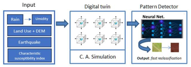
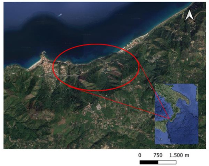
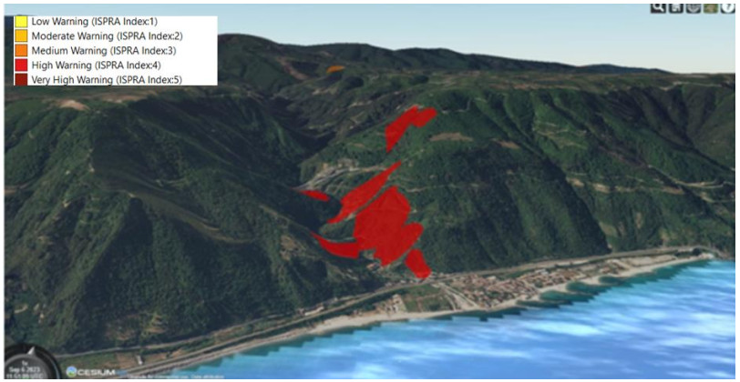
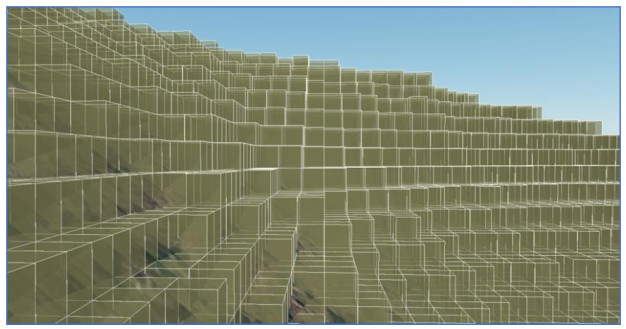
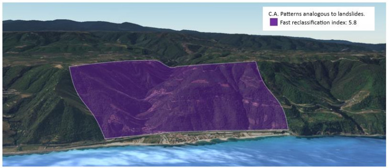
Landslides represent a growing threat among the various morphological processes that cause damage to territories. To address this problem and prevent the associated risks, it is essential to quickly find adequate methodologies capable of predicting these phenomena in advance. The following study focuses on the implementation of an experimental WebGIS infrastructure designed and built to predict the susceptibility index of a specific presumably at-risk area in real time (using specific input data) and in response to extreme weather events (such as heavy rain). The climate data values are calculated through an innovative and experimental atmospheric simulator developed by the authors, which is capable of providing data on meteorological variables with high spatial precision. To this end, the terrain is represented through cellular automata, implementing a suitable neural network useful for producing the desired output. The effectiveness of this methodology was tested on two debris flow events that occurred in the Calabria region, specifically in the province of Reggio Calabria, in 2001 and 2005, which caused extensive damage. The (forecast) results obtained with the proposed methodology were compared with the (known) historical data, confirming the effectiveness of the method in predicting (and therefore signaling the possibility of an imminent landslide event) a higher susceptibility index than the known one and one provided (to date) by the Higher Institute for Environmental Protection and Research (ISPRA), validating the result obtained through the actual subsequent occurrence of a landslide event in the area under investigation. Therefore, the method proposed today is not aimed at predicting the local movement of a small landslide area, but is primarily aimed at predicting the change or improving the variation of the landslide susceptibility index to compare the predicted value with the current one provided by the relevant bodies (ISPRA), thus signaling an alert for the entire area under investigation.
Citation: Vincenzo Barrile, Emanuela Genovese, Francesco Cotroneo. Geomatics, soft computing, and innovative simulator: prediction of susceptibility to landslide risk[J]. AIMS Geosciences, 2024, 10(2): 399-418. doi: 10.3934/geosci.2024021
Landslides represent a growing threat among the various morphological processes that cause damage to territories. To address this problem and prevent the associated risks, it is essential to quickly find adequate methodologies capable of predicting these phenomena in advance. The following study focuses on the implementation of an experimental WebGIS infrastructure designed and built to predict the susceptibility index of a specific presumably at-risk area in real time (using specific input data) and in response to extreme weather events (such as heavy rain). The climate data values are calculated through an innovative and experimental atmospheric simulator developed by the authors, which is capable of providing data on meteorological variables with high spatial precision. To this end, the terrain is represented through cellular automata, implementing a suitable neural network useful for producing the desired output. The effectiveness of this methodology was tested on two debris flow events that occurred in the Calabria region, specifically in the province of Reggio Calabria, in 2001 and 2005, which caused extensive damage. The (forecast) results obtained with the proposed methodology were compared with the (known) historical data, confirming the effectiveness of the method in predicting (and therefore signaling the possibility of an imminent landslide event) a higher susceptibility index than the known one and one provided (to date) by the Higher Institute for Environmental Protection and Research (ISPRA), validating the result obtained through the actual subsequent occurrence of a landslide event in the area under investigation. Therefore, the method proposed today is not aimed at predicting the local movement of a small landslide area, but is primarily aimed at predicting the change or improving the variation of the landslide susceptibility index to compare the predicted value with the current one provided by the relevant bodies (ISPRA), thus signaling an alert for the entire area under investigation.

| [1] |
Gu T, Duan P, Wang M, et al. (2024) Effects of non-landslide sampling strategies on machine learning models in landslide susceptibility mapping. Sci Rep 14: 7201. https://doi.org/10.1038/s41598-024-57964-5 doi: 10.1038/s41598-024-57964-5

|
| [2] |
Nwazelibe VE, Egbueri JC, Unigwe CO, et al. (2023) GIS-based landslide susceptibility mapping of Western Rwanda: an integrated artificial neural network, frequency ratio, and Shannon entropy approach. Environ Earth Sci 82: 439. https://doi.org/10.1007/s12665-023-11134-4 doi: 10.1007/s12665-023-11134-4
|
| [3] | Unigwe CO, Egbueri JC, Omeka ME, et al. (2023). Landslide Occurrences in Southeastern Nigeria: A Literature Analysis on the Impact of Rainfall. In: Egbueri JC, Ighalo JO, Pande CB (eds), Climate Change Impacts on Nigeria. Springer Climate. Springer, Cham. https://doi.org/10.1007/978-3-031-21007-5_18 |
| [4] |
Nwazelibe VE, Unigwe CO, Egbueri JC (2023) Testing the performances of different fuzzy overlay methods in GIS-based landslide susceptibility mapping of Udi Province, SE Nigeria. Catena 20: 106654. https://doi.org/10.1016/j.catena.2022.106654 doi: 10.1016/j.catena.2022.106654
|
| [5] |
Nwazelibe VE, Unigwe CO, Egbueri JC (2023) Integration and comparison of algorithmic weight of evidence and logistic regression in landslide susceptibility mapping of the Orumba North erosion-prone region, Nigeria. Model Earth Syst Environ 9: 967–986. https://doi.org/10.1007/s40808-022-01549-6 doi: 10.1007/s40808-022-01549-6
|
| [6] | ISPRA, Istituto Superiore per la Protezione e la Ricerca Amabientale. Available from: https://indicatoriambientali.isprambiente.it/sys_ind/report/html/737#C737. |
| [7] | ISPRA. Rapporto Frane, Capitolo 23 Calabria. Available from: https://www.isprambiente.gov.it/files/pubblicazioni/rapporti/rapporto-frane/capitolo-23-calabria.pdf. |
| [8] | ISPRA. Repporto Frane, Capitolo 4 WebGIS. Available from: https://www.isprambiente.gov.it/files/pubblicazioni/rapporti/rapporto-frane/capitolo-4-webgis.pdf. |
| [9] | Inventario Frane IFFI. IdroGEO. Available from: https://idrogeo.isprambiente.it/app/iffi/f/0801267600?@ = 38.25051188109998, 15.753338061897404, 16. |
| [10] |
Mondini AC, Guzzetti F, Melillo M (2023) Deep learning forecast of rainfall-induced shallow landslides. Nat Commun 14: 1–10. https://doi.org/10.1038/s41467-023-38135-y doi: 10.1038/s41467-023-38135-y
|
| [11] |
Moraci N, Mandaglio MC, Gioffrè D, et al. (2017) Debris flow susceptibility zoning: an approach applied to a study area. Riv Ital Geotec 51: 47–62. https://doi.org/10.19199/2017.2.0557-1405.047 doi: 10.19199/2017.2.0557-1405.047
|
| [12] |
Borrelli L, Ciurleo M, Gullà G (2018) Shallow landslide susceptibility assessment in granitic rocks using GIS-based statistical methods: the contribution of the weathering grade map. Landslides 15: 1127–1142. https://doi.org/10.1007/s10346-018-0947-7 doi: 10.1007/s10346-018-0947-7
|
| [13] |
Cascini L, Ciurleo M, Di Nocera S, et al. (2015) A new–old approach for shallow landslide analysis and susceptibility zoning in fine-grained weathered soils of southern Italy. Geomorphology 241: 371–381. https://doi.org/10.1016/j.geomorph.2015.04.017 doi: 10.1016/j.geomorph.2015.04.017
|
| [14] |
Ciurleo M, Ferlisi S, Foresta V, et al. (2022) Landslide Susceptibility Analysis by Applying TRIGRS to a Reliable Geotechnical Slope Model. Geosciences 12: 18. https://doi.org/10.3390/geosciences12010018 doi: 10.3390/geosciences12010018
|
| [15] | Ferlisi S, De Chiara G (2018) Risk analysis for rainfall-induced slope instabilities in coarse-grained soils: Practice and perspectives in Italy. In Landslides and engineered slopes. Experience, theory and practice. CRC Press. 137–154. https://doi.org/10.1201/9781315375007-8 |
| [16] | Spizzichino D, Margottini C, Trigila A, et al. (2013) Landslide impacts in Europe: Weaknesses and strengths of databases available at European and national scale. In: Margottini C, Canuti P, Sassa K (eds), Landslide Science and Practice, Volume 1: Landslide Inventory and Susceptibility and Hazard Zoning, 73–80. https://doi.org/10.1007/978-3-642-31325-7_9 |
| [17] | Barrile V, Cotroneo F, Iorio F, et al. (2022) An Innovative Experimental Software for Geomatics Applications on the Environment and the Territory. In Italian Conference on Geomatics and Geospatial Technologies. Cham: Springer International Publishing, 102–113. https://doi.org/10.1007/978-3-031-17439-1_7 |
| [18] |
Bilotta G, Genovese E, Citroni R, et al. (2023) Integration of an Innovative Atmospheric Forecasting Simulator and Remote Sensing Data into a Geographical Information System in the Frame of Agriculture 4.0 Concept. AgriEngineering 5: 1280–1301. https://doi.org/10.3390/agriengineering5030081 doi: 10.3390/agriengineering5030081
|
| [19] |
Bonavina M, Bozzano F, Martino S, et al. (2005) Le colate di fango e detrito lungo il versante costiero tra Bagnara Calabra e Scilla (Reggio Calabria): valutazioni di suscettibilità. G Geol Appl 2: 65–74. https://doi.org/10.1474/GGA.2005–02.0–09.0035 doi: 10.1474/GGA.2005–02.0–09.0035
|
| [20] | Reichenbach P, Busca C, Mondini AC, et al. (2015) Land use change scenarios and landslide susceptibility zonation: The briga catchment test area (Messina, Italy). In Lollino G, Manconi A, Clague J, et al. (eds), Engineering Geology for Society and Territory-Volume 1: Climate Change and Engineering Geology. Springer International Publishing, 557–561. |
| [21] |
Bhattacharjee K, Naskar N, Roy S, et al. (2020) A survey of cellular automata: types, dynamics, non-uniformity, and applications. Natural Comput 19: 433–461. https://doi.org/10.1007/s11047-018-9696-8 doi: 10.1007/s11047-018-9696-8
|
| [22] |
Hun LD, Min KD, Mo JJ (2020) A Unity-based Simulator for Tsunami Evacuation with DEVS Agent Model and Cellular Automata. J Korea Multimedia Soc 23: 772–783. https://doi.org/10.9717/kmms.2020.23.6.772 doi: 10.9717/kmms.2020.23.6.772
|
| [23] |
Sachidananda M, Zrnić DS (1987) Rain rate estimates from differential polarization measurements. J Atmos Oceanic Technol 4: 588–598. https://doi.org/10.1175/1520-0426(1987)004<0588:RREFDP>2.0.CO;2 doi: 10.1175/1520-0426(1987)004<0588:RREFDP>2.0.CO;2
|
| [24] |
Kale RV, Sahoo B (2011) Green-Ampt infiltration models for varied field conditions: A revisit. Water Resour Manage 25: 3505–3536. https://doi.org/10.1007/s11269-011-9868-0 doi: 10.1007/s11269-011-9868-0
|
| [25] | Klambauer G, Unterthiner T, Mayr A, et al. (2017) Self-normalizing neural networks. In Advances in Neural Information Processing Systems 30. |
| [26] |
Zhang D, Yang J, Li F, et al. (2022) Landslide risk prediction model using an attention-based temporal convolutional network connected to a recurrent neural network. IEEE Access 10: 37635–37645. https://doi.org/10.1109/ACCESS.2022.3165051 doi: 10.1109/ACCESS.2022.3165051
|
| [27] |
Vacondio R, Altomare C, De Leffe M, et al. (2021) Grand challenges for smoothed particle hydrodynamics numerical schemes. Comput Part Mech 8: 575–588. https://doi.org/10.1007/s40571-020-00354-1 doi: 10.1007/s40571-020-00354-1
|
| [28] | Barrile V, Bilotta G, Fotia A (2018) Analysis of hydraulic risk territories: comparison between LIDAR and other different techniques for 3D modeling. WSEAS Trans Environ Dev 14: 45–52. |
| [29] |
Wang S, Zhang K, van Beek LPH, et al. (2020) Physically based landslide prediction over a large region: scaling low-resolution hydrological model results for high resolution slope stability assessment. Environ Model Softw 124: 104607. https://doi.org/10.1016/j.envsoft.2019.104607 doi: 10.1016/j.envsoft.2019.104607
|
| [30] | Italian National Geoportal Viewer. Available from: http://www.pcn.minambiente.it/viewer/. |
| [31] |
Yao J, Yao X, Liu X (2022) Landslide Detection and Mapping Based on SBAS-InSAR and PS-InSAR: A Case Study in Gongjue County, Tibet, China. Remote Sens 14: 4728. https://doi.org/10.3390/rs14194728 doi: 10.3390/rs14194728
|
| [32] | La Guardia M, Koeva M, D'ippolito F, et al. (2022) 3D Data integration for web based open source WebGL interactive visualisation. In 17th 3D GeoInfo Conference, 89–94. https://doi.org/10.5194/isprs-archives-XLVIII-4-W4-2022-89-2022 |
Figures(10)

Vincenzo Barrile, Emanuela Genovese, Francesco Cotroneo. Geomatics, soft computing, and innovative simulator: prediction of susceptibility to landslide risk[J]. AIMS Geosciences, 2024, 10(2): 399-418. doi: 10.3934/geosci.2024021


 DownLoad: