Landscape mapping using ground-penetrating radar, electrical resistivity tomography survey and landscape profiling

Victor M Matasov; Svetlana S Bricheva; Alexey A Bobachev; Iya V Mironenko; Anton V Fedin; Vladislav V Sysuev; Lyudmila A Zolotaya; Sergey B Roganov; Victor M Matasov; Svetlana S Bricheva; Alexey A Bobachev; Iya V Mironenko; Anton V Fedin; Vladislav V Sysuev; Lyudmila A Zolotaya; Sergey B Roganov

doi:10.3934/geosci.2022012

AIMS Geosciences

2022, Volume 8, Issue 2: 213-223. doi: 10.3934/geosci.2022012

Previous Article Next Article

Research article Special Issues

Landscape mapping using ground-penetrating radar, electrical resistivity tomography survey and landscape profiling

1.
Department of Landscape Design and Sustainable Ecosystems, Agrarian-Technological Institute, Peoples' Friendship University of Russia—RUDN University, Moscow, Russia
2.
Department of Physical Geography and Landscape Science, Faculty of Geography, Lomonosov MSU, Moscow, Russia
3.
Faculty of Geography and Geoinformation Technology, Higher School of Economics, Moscow, Russia
4.
Department of Seismic and Geoacoustic, Faculty of Geology, Lomonosov MSU, Moscow, Russia
5.
Department of Quaternary paleogeography, Institute of Geography RAS, Moscow, Russia
6.
Department of Geology and Geophysics NSU, Novosibirsk, Russia
7.
Department of Geophysical Methods of Earth Crust Study, Faculty of Geology, Lomonosov MSU, Moscow, Russia
8.
Laboratory of Geomorphology, Institute of Geography RAS, Moscow, Russia

Received: 04 December 2021 Revised: 12 January 2022 Accepted: 08 February 2022 Published: 23 February 2022

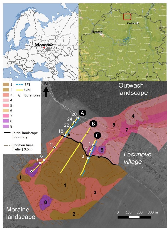
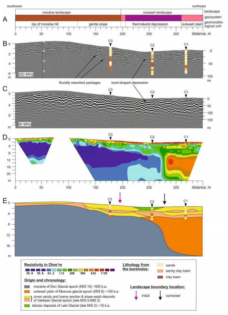
This work aims to verify and correct the boundary between two landscapes—moraine and outwash plain—delineated earlier by the classical landscape approach. The initial interpretation of the boundary caused controversy due to the appearance of the thermokarst depression in the outwash landscape. The lithological structure is one of the main factors of landscape differentiation. The classical approach includes drilling to obtain the lithological and sedimentary data. However, the boreholes are usually shallow, while geophysical methods allow to look deeper into the subsurface and improve our knowledge about lithological structure and stratigraphy. In this study, we use ground-penetrating radar with a peak frequency of 250 and 50 MHz and detailed electrical resistivity tomography (with 1 m electrode spacing) in addition to the landscape mapping and drilling to correct the landscape boundary position. We conclude that it is primarily defined by the subsurface boundary between lithological complexes of clayish moraine deposits and sandy outwash deposits located at 7 m depth. Moving the boundary to the northeast by 70–100 m from the current position removes inconsistencies and clarifies the history of the area's formation in the Quaternary.
- critical zones,
- geophysical methods,
- landscape studies,
- Meshchyora lowlands
Citation: Victor M Matasov, Svetlana S Bricheva, Alexey A Bobachev, Iya V Mironenko, Anton V Fedin, Vladislav V Sysuev, Lyudmila A Zolotaya, Sergey B Roganov. Landscape mapping using ground-penetrating radar, electrical resistivity tomography survey and landscape profiling[J]. AIMS Geosciences, 2022, 8(2): 213-223. doi: 10.3934/geosci.2022012

Related Papers:

Abstract

This work aims to verify and correct the boundary between two landscapes—moraine and outwash plain—delineated earlier by the classical landscape approach. The initial interpretation of the boundary caused controversy due to the appearance of the thermokarst depression in the outwash landscape. The lithological structure is one of the main factors of landscape differentiation. The classical approach includes drilling to obtain the lithological and sedimentary data. However, the boreholes are usually shallow, while geophysical methods allow to look deeper into the subsurface and improve our knowledge about lithological structure and stratigraphy. In this study, we use ground-penetrating radar with a peak frequency of 250 and 50 MHz and detailed electrical resistivity tomography (with 1 m electrode spacing) in addition to the landscape mapping and drilling to correct the landscape boundary position. We conclude that it is primarily defined by the subsurface boundary between lithological complexes of clayish moraine deposits and sandy outwash deposits located at 7 m depth. Moving the boundary to the northeast by 70–100 m from the current position removes inconsistencies and clarifies the history of the area's formation in the Quaternary.

References

[1]	Fan B, Liu X, Zhu Q, et al. (2020) Exploring the interplay between infiltration dynamics and Critical Zone structures with multiscale geophysical imaging: A review. Geoderma 374: 114431. https://doi.org/10.1016/j.geoderma.2020.114431 doi: 10.1016/j.geoderma.2020.114431
[2]	Chorover J, Kretzschmar R, Garcia-Pichel F, et al. (2007) Soil Biogeochemical Processes within the Critical Zone. Elements 3: 321-326. https://doi.org/10.2113/gselements.3.5.321 doi: 10.2113/gselements.3.5.321
[3]	Frolova M (2019) From the Russian/Soviet landscape concept to the geosystem approach to integrative environmental studies in an international context. Landscape Ecol 34: 1485-1502. https://doi.org/10.1007/s10980-018-0751-8 doi: 10.1007/s10980-018-0751-8
[4]	Solntsev NA (1948) The natural geographic landscape and some of its general rules. Proc Second All-Union Geogr Congr 1: 258-269.
[5]	Bryan BA (2003) Physical environmental modeling, visualization and query for supporting landscape planning decisions. Landscape Urban Plann 65: 237-259. https://doi.org/10.1016/S0169-2046(03)00059-8 doi: 10.1016/S0169-2046(03)00059-8
[6]	Opdam P, Luque S, Nassauer J, et al. (2018) How can landscape ecology contribute to sustainability science? Landscape Ecol 33: 1-7. https://doi.org/10.1007/s10980-018-0610-7 doi: 10.1007/s10980-018-0610-7
[7]	Alekseeva NN, Klimanova OA, Khazieva ES (2017) Global land cover data bases and their perspectives for present-day landscapes mapping. Izvestiya RAN Ser Geogr, 110-123. https://doi.org/10.15356/0373-2444-2017-1-110-123 doi: 10.15356/0373-2444-2017-1-110-123
[8]	Lavalle C, Baranzelli C, Batista e Silva F, et al. (2011) A High Resolution Land Use/Cover Modelling Framework for Europe: Introducing the EU-ClueScanner100 Model, Computational Science and Its Applications ICCSA 2011, Berlin, Heidelberg, Springer, 60-75.
[9]	Bristow CS, Jol HM (2003) Ground penetrating radar in sediments, London, Geological Society. https://doi.org/10.1144/GSL.SP.2003.211
[10]	Bricheva SS, Modin IN, Panin AV, et al. (2020) The Structure of Quaternary Deposits in the Upper Dnieper Valley According to Integrated (Combined) Geophysical Data. Moscow Univ Geol Bull 75: 413-424. https://doi.org/10.3103/S014587522004002X doi: 10.3103/S014587522004002X
[11]	Pellicer XM, Gibson P (2011) Electrical resistivity and Ground Penetrating Radar for the characterisation of the internal architecture of Quaternary sediments in the Midlands of Ireland. J Appl Geophys 75: 638-647. https://doi.org/10.1016/j.jappgeo.2011.09.019 doi: 10.1016/j.jappgeo.2011.09.019
[12]	Conyers LB (2018) Ground-penetrating Radar and Magnetometry for Buried Landscape Analysis, Cham, Springer International Publishing.
[13]	Ryazantsev PA, Bakhmet ON (2020) Application of Geoelectric Methods for Mapping Soil Heterogeneity. Eurasian Soil Sc 53: 558-568. https://doi.org/10.1134/S1064229320050129 doi: 10.1134/S1064229320050129
[14]	Zolotaya LA, Kosnyreva MV (2015) Ground-penetrating radar (GPR) researches in solving soil geophysics problems. Geofizika 2: 16-22.
[15]	Martin T, Nordsiek S, Weller A (2015) Low-Frequency Impedance Spectroscopy of Wood. J Res Spectrosc 2015: 9.
[16]	Bricheva SS, Matasov VM, Shilov PM (2017) Ground penetrating radar (GPR) as a part of integrated landscape studies on peatlands. Geoecol Eng geol Hydrogeol Geocryology 3: 76-83.
[17]	Sysuev VV (2014) Geo-radar investigation of the poly-scale structures in landscapes (case study of the Smolensk-Moscow highland). Vestnik Mosk Univ Seriya 5 Geografiya 4: 26-33.
[18]	Mamay Ⅱ (1992) Dinamika landshaftov. Metodika izucheniya, Moskva, Izd-vo Mosk. un-ta. Available from: https://search.rsl.ru/ru/record/01001639692
[19]	Novenko EY, Tsyganov AN, Volkova EM, et al. (2016) Mid- and Late Holocene vegetation dynamics and fire history in the boreal forest of European Russia: A case study from Meshchera Lowlands. Palaeogeogr Palaeoclimatol Palaeoecol 459: 570-584. https://doi.org/10.1016/j.palaeo.2016.08.004 doi: 10.1016/j.palaeo.2016.08.004
[20]	Matasov V, Prishchepov AV, Jepsen MR, et al. (2019) Spatial determinants and underlying drivers of land-use transitions in European Russia from 1770 to 2010. J Land Use Sci 14: 362-377. https://doi.org/10.1080/1747423X.2019.1709224 doi: 10.1080/1747423X.2019.1709224
[21]	Aseev AA, Vedenskaya IE (1962) Razvitie rel'efa Meshcherskoj nizmennosti, Moskva, Izd-vo AN SSSR. Available from: https://search.rsl.ru/ru/record/01005950799
[22]	Mamay Ⅱ (2013) Zakonomernosti projavlenija processov v landshaftah Meshhjory. Landshaftnyj sbornik (Razvitie idej N.A. Solnceva v sovremennom landshaftovedenii). M Smolensk: Ojkumena, 32-34. Available from: https://elibrary.ru/item.asp?id=25180335
[23]	Dahlin T, Zhou B (2004) A numerical comparison of 2D resistivity imaging with 10 electrode arrays. Geophys Prospect 52: 379-398. https://doi.org/10.1111/j.1365-2478.2004.00423.x doi: 10.1111/j.1365-2478.2004.00423.x
[24]	Astakhov V, Shkatova V, Zastrozhnov A, et al. (2016) Glaciomorphological Map of the Russian Federation. Quat Int 420: 4-14. https://doi.org/10.1016/j.quaint.2015.09.024 doi: 10.1016/j.quaint.2015.09.024
[25]	Kupriyanov DA, Novenko EY (2019) Reconstruction of the Holocene Dynamics of Forest Fires in the Central Part of Meshcherskaya Lowlands According to Antracological Analysis. Contemp Probl Ecol 12: 204-212. https://doi.org/10.1134/S1995425519030065 doi: 10.1134/S1995425519030065
[26]	Novenko EY, Mironenko IV, Kupriyanov DA, et al. (2019) Pre-agrarian landscapes in Southeastern Meshchera: reconstruction from paleoecological data. Geogr Nat Res. Available from: https://elibrary.ru/item.asp?id=37418763&

Reader Comments

Your name:*

Email:*
© 2022 the Author(s), licensee AIMS Press. This is an open access article distributed under the terms of the Creative Commons Attribution License (http://creativecommons.org/licenses/by/4.0)