Hopf bifurcation induced by fear: A Leslie-Gower reaction-diffusion predator-prey model

Jiani Jin; Haokun Qi; Bing Liu; Jiani Jin; Haokun Qi; Bing Liu

doi:10.3934/era.2024304

Electronic Research Archive

2024, Volume 32, Issue 12: 6503-6534. doi: 10.3934/era.2024304

Previous Article Next Article

Research article Special Issues

Hopf bifurcation induced by fear: A Leslie-Gower reaction-diffusion predator-prey model

1.
School of Mathematics, Anshan Normal University, Anshan Liaoning 114007, China
2.
School of Mathematics, Liaoning Normal University, Dalian Liaoning 116029, China

Received: 17 October 2024 Revised: 15 November 2024 Accepted: 22 November 2024 Published: 02 December 2024

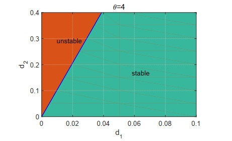
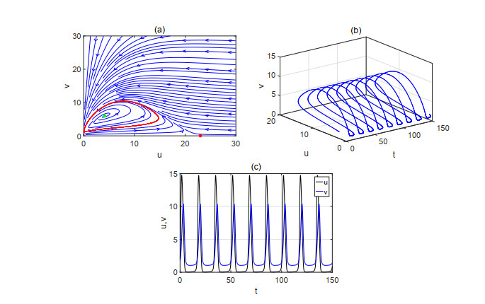
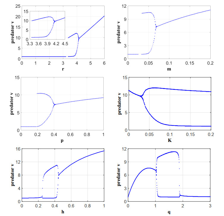
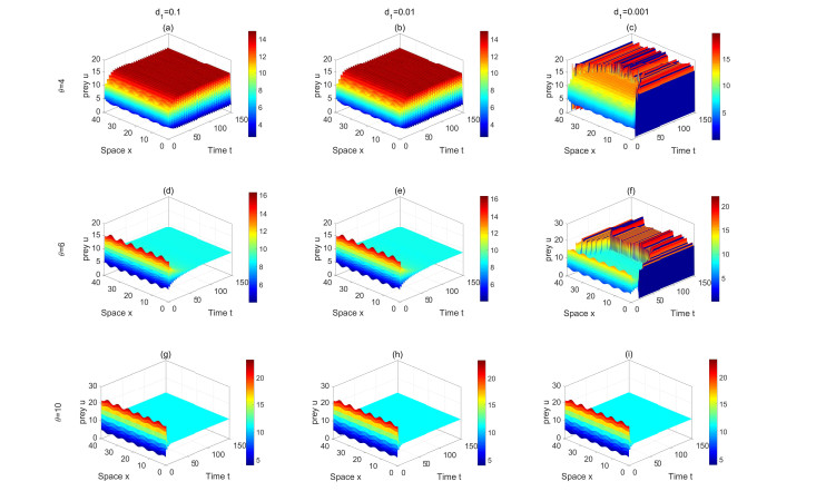
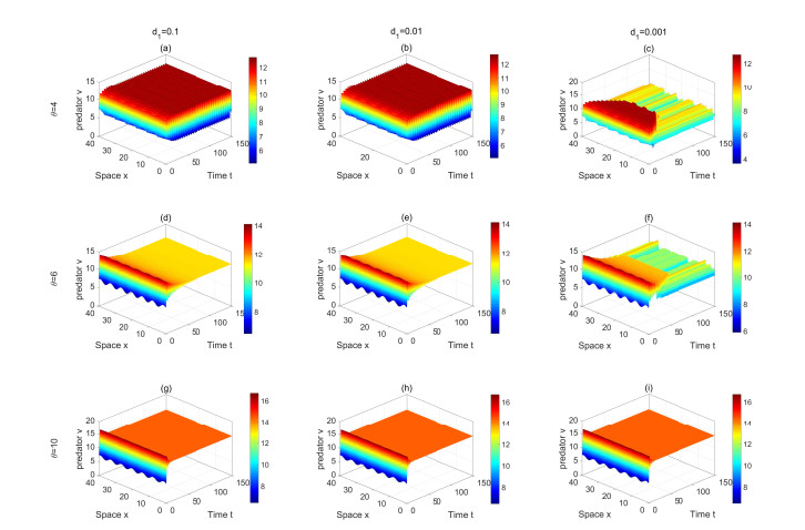
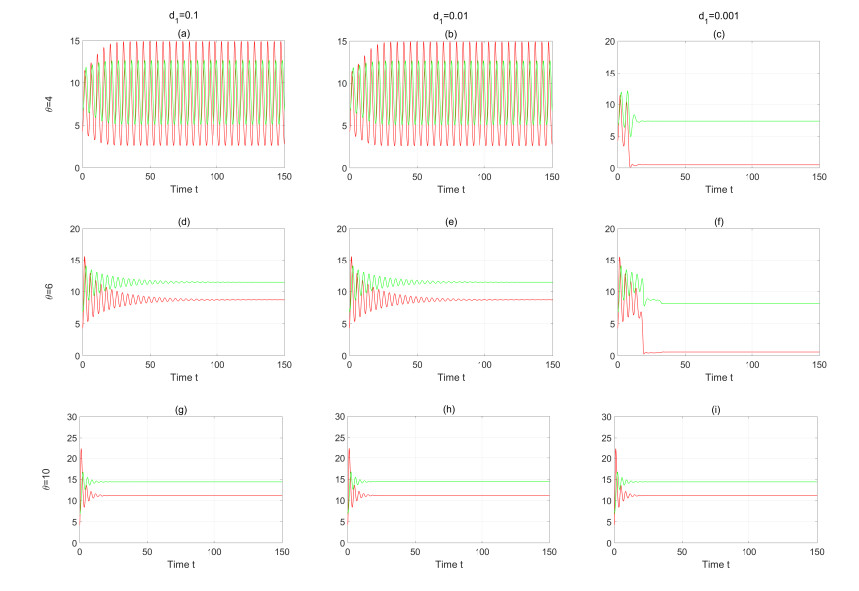
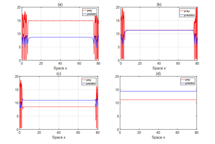
The aim of this paper was to explore the impact of fear on the dynamics of prey and predator species. Specifically, we investigated a reaction-diffusion predator-prey model in which the prey was subjected to Beddington-DeAngelis type and the predator was subjected to modified Leslie-Gower type. First, we analyzed the existence and stability of equilibria of the nonspatial model, and further investigated the global stability and Hopf bifurcation at the unique positive equilibrium point. For the spatial model, we studied the local and global stability of the unique constant positive steady state solution and captured the existence of Turing instability, which depended on the diffusion rate ratio between the two species. Then, we demonstrated the existence of Hopf bifurcations and discussed the direction and stability of spatially homogeneous and inhomogeneous periodic solutions. Finally, the impact of fear and spatial diffusion on the dynamics of populations were probed by numerical simulations. Results revealed that spatial diffusion and fear both broaden the dynamical properties of this model, facilitating the emergence of periodic solutions and the formation of biodiversity.
- predator-prey model,
- reaction-diffusion,
- fear effect,
- Turing instability,
- Hopf bifurcation
Citation: Jiani Jin, Haokun Qi, Bing Liu. Hopf bifurcation induced by fear: A Leslie-Gower reaction-diffusion predator-prey model[J]. Electronic Research Archive, 2024, 32(12): 6503-6534. doi: 10.3934/era.2024304

Related Papers:

Abstract

The aim of this paper was to explore the impact of fear on the dynamics of prey and predator species. Specifically, we investigated a reaction-diffusion predator-prey model in which the prey was subjected to Beddington-DeAngelis type and the predator was subjected to modified Leslie-Gower type. First, we analyzed the existence and stability of equilibria of the nonspatial model, and further investigated the global stability and Hopf bifurcation at the unique positive equilibrium point. For the spatial model, we studied the local and global stability of the unique constant positive steady state solution and captured the existence of Turing instability, which depended on the diffusion rate ratio between the two species. Then, we demonstrated the existence of Hopf bifurcations and discussed the direction and stability of spatially homogeneous and inhomogeneous periodic solutions. Finally, the impact of fear and spatial diffusion on the dynamics of populations were probed by numerical simulations. Results revealed that spatial diffusion and fear both broaden the dynamical properties of this model, facilitating the emergence of periodic solutions and the formation of biodiversity.

References

[1]	K. B. Altendorf, J. W. Laundré, C. A. L. González, J. S. Brown, Assessing effects of predation risk on foraging behavior of mule deer, J. Mammal., 82 (2001), 430–439.
[2]	S. Creel, D. Christianson, S. Liley, J. A. Winnie, Predation risk affects reproductive physiology and demography of Elk, Science, 315 (2007), 960. https://doi.org/10.1126/science.1135918 doi: 10.1126/science.1135918
[3]	W. Cresswell, Predation in bird populations, J. Ornithol., 152 (2011), 251–263. https://doi.org/10.1007/s10336-010-0638-1 doi: 10.1007/s10336-010-0638-1
[4]	L. Y. Zanette, A. F. White, M. C. Allen, M. Clinchy, Perceived predation risk reduces the number of offspring songbirds produce per year, Science, 334 (2011), 1398–1401. https://doi.org/10.1126/science.1210908 doi: 10.1126/science.1210908
[5]	K. Sarkara, S. Khajanchi, Impact of fear effect on the growth of prey in a predator-prey interaction model, Ecol. Complexity, 42 (2020), 100826. https://doi.org/10.1016/j.ecocom.2020.100826 doi: 10.1016/j.ecocom.2020.100826
[6]	C. S. Holling, The functional response of invertebrate predators to prey density, Mem. Entomol. Soc. Can., 98 (1966), 5–86. https://doi.org/10.4039/entm9848fv doi: 10.4039/entm9848fv
[7]	J. R. Beddington, Mutual interference between parasites or predators and its effect on searching efficiency, J. Anim. Ecol., 44 (1975), 331–340. https://doi.org/10.2307/3866 doi: 10.2307/3866
[8]	D. L. DeAngelis, R. A. Goldstein, R. V. O'neill, A model for tropic interaction, Ecology, 56 (1975), 881–892. https://doi.org/10.2307/1936298 doi: 10.2307/1936298
[9]	P. H. Leslie, J. G. Gower, The properties of a stochastic model for the predator-prey type of interaction between two species, Biometrika, 47 (1960), 219–234. https://doi.org/10.2307/2333294 doi: 10.2307/2333294
[10]	J. Huang, X. Xia, X. Zhang, S. Ruan, Bifurcation of Codimension 3 in a Predator-Prey System of Leslie Type with Simplified Holling Type Ⅳ Functional Response, Int. J. Bifurcation Chaos, 26 (2016), 1650034. https://doi.org/10.1142/S0218127416500346 doi: 10.1142/S0218127416500346
[11]	W. Ko, K. Ryu, Qualitative analysis of a predator-prey model with Holling type Ⅱ functional response incorporating a prey refuge, J. Differ. Equations, 231 (2006), 534–550. https://doi.org/10.1016/j.jde.2006.08.001 doi: 10.1016/j.jde.2006.08.001
[12]	X. Wang, L. Zanette, X. Zou, Modelling the fear effect in predator-prey interactions, J. Math. Biol., 73 (2016), 1179–1204. https://doi.org/10.1007/s00285-016-0989-1 doi: 10.1007/s00285-016-0989-1
[13]	S. Pal, S. Majhi, S. Mandal, N. Pal, Role of fear in a predator-prey model with Beddington-Deangelis functional response, Z. Naturforsch. A, 74 (2019), 581–595. https://doi.org/10.1515/zna-2018-0449 doi: 10.1515/zna-2018-0449
[14]	J. Wang, Y. Cai, S. Fu, W. Wang, The effect of the fear factor on the dynamics of a predator-prey model incorporating the prey refuge, Chaos, 29 (2019), 083109. https://doi.org/10.1063/1.5111121 doi: 10.1063/1.5111121
[15]	A. M. Turing, The chemical basis of morphogenesis, Philos. Trans. R. Soc., B., 237 (1952), 37–72. https://doi.org/10.1098/rstb.1952.0012 doi: 10.1098/rstb.1952.0012
[16]	Y. Song, X. Tang, Stability, steady-state bifurcations, and turing patterns in a predator–prey model with herd behavior and prey-taxis, Stud. Appl. Math., 139 (2017), 371–404. https://doi.org/10.1111/sapm.12165 doi: 10.1111/sapm.12165
[17]	S. Yan, D. Jia, T. Zhang, S. Yuan, Pattern dynamics in a diffusive predator-prey model with hunting cooperations, Chaos Solitons Fractals, 130 (2020), 109428. https://doi.org/10.1016/j.chaos.2019.109428 doi: 10.1016/j.chaos.2019.109428
[18]	R. Peng, J. Shi, Non-existence of non-constant positive steady states of two Holling type-Ⅱ predator-prey systems: strong interaction case, J. Differ. Equations, 247 (2009), 866–886. https://doi.org/10.1016/j.jde.2009.03.008 doi: 10.1016/j.jde.2009.03.008
[19]	J. Wang, J. Wei, J. Shi, Global bifurcation analysis and pattern formation in homogeneous diffusive predator-prey systems, J. Differ. Equations, 260 (2016), 3495–3523. https://doi.org/10.1016/j.jde.2015.10.036 doi: 10.1016/j.jde.2015.10.036
[20]	M. Chen, Pattern dynamics of a Lotka-Volterra model with taxis mechanism, Appl. Math. Comput., 484 (2025), 129017. https://doi.org/10.1016/j.amc.2024.129017 doi: 10.1016/j.amc.2024.129017
[21]	R. Han, L. N. Guin, B. Dai, Cross-diffusion-driven pattern formation and selection in a modified Leslie-Gower predator-prey model with fear effect, J. Biol. Syst., 28 (2020), 27–64. https://doi.org/10.1142/S0218339020500023 doi: 10.1142/S0218339020500023
[22]	V. Tiwari, J. P. Tripathi, S. Mishra, R. K. Upadhyay, Modeling the fear effect and stability of non-equilibrium patterns in mutually interfering predator-prey systems, Appl. Math. Comput., 371 (2020), 124948. https://doi.org/10.1016/j.amc.2019.124948 doi: 10.1016/j.amc.2019.124948
[23]	T. Zhang, T. Zhang, X. Meng, Stability analysis of a chemostat model with maintenance energy, Appl. Math. Lett., 68 (2017), 1–7. https://doi.org/10.1016/j.aml.2016.12.007 doi: 10.1016/j.aml.2016.12.007
[24]	F. Yi, J. Wei, J. Shi, Bifurcation and spatiotemporal patterns in a homogeneous diffusive predator-prey system, J. Differ. Equations, 246 (2009), 1944–1977. https://doi.org/10.1016/j.jde.2008.10.024 doi: 10.1016/j.jde.2008.10.024
[25]	B. D. Hassard, N. D. Kazarinoff, Y. Wan, Theory and Applications of Hopf Bifurcation, Cambridge University Press, Cambridge, 1981.
[26]	M. Liu, E. Liz, G. Röst, Endemic bubbles generated by delayed behavioral response: Global stability and bifurcation switches in an SIS model, SIAM J. Appl. Math., 75 (2015), 75–91. https://doi.org/10.1137/140972652 doi: 10.1137/140972652
[27]	X. Wang, Y. Tan, Y. Cai, W. Wang, Impact of the fear effect on the stability and bifurcation of a leslie-gower predator-prey model, Int. J. Bifurcation Chaos, 30 (2020), 2050210. https://doi.org/10.1142/S0218127420502107 doi: 10.1142/S0218127420502107

Reader Comments

Your name:*

Email:*
© 2024 the Author(s), licensee AIMS Press. This is an open access article distributed under the terms of the Creative Commons Attribution License (http://creativecommons.org/licenses/by/4.0)