Dynamical analysis of a heterogeneous spatial diffusion Zika model with vector-bias and environmental transmission

Liping Wang; Xinyu Wang; Dajun Liu; Xuekang Zhang; Peng Wu; Liping Wang; Xinyu Wang; Dajun Liu; Xuekang Zhang; Peng Wu

doi:10.3934/era.2024061

Electronic Research Archive

2024, Volume 32, Issue 2: 1308-1332. doi: 10.3934/era.2024061

Previous Article Next Article

Research article

Dynamical analysis of a heterogeneous spatial diffusion Zika model with vector-bias and environmental transmission

1.
School of Mathematics-Physics and Finance, Anhui Polytechnic University, Wuhu 241000, China
2.
School of Sciences, Hangzhou Dianzi University, Hangzhou 310018, China

Academic Editor: Pengcheng Xiao

Received: 05 November 2023 Revised: 03 January 2024 Accepted: 26 January 2024 Published: 31 January 2024

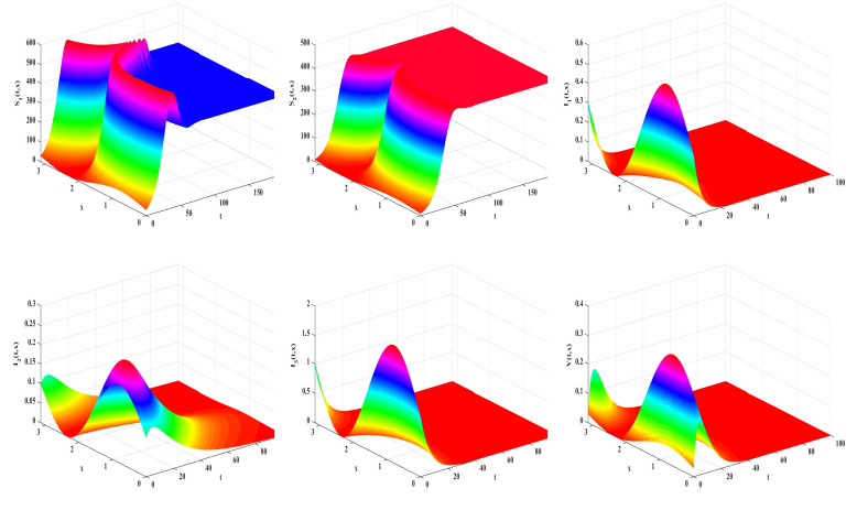
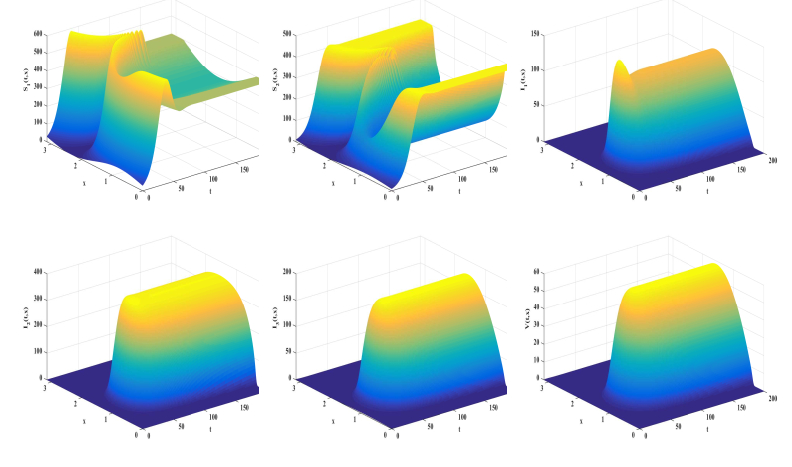
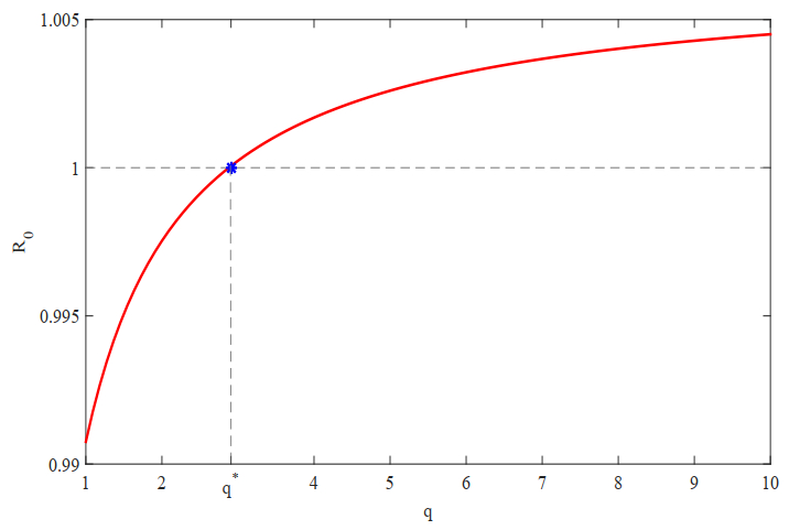
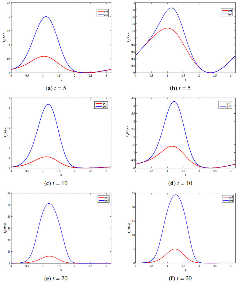
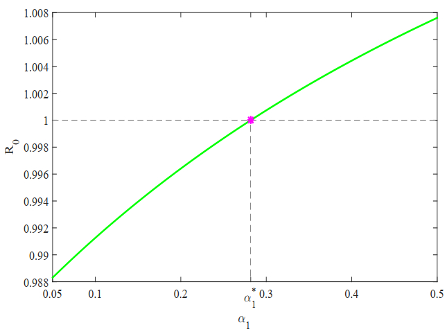
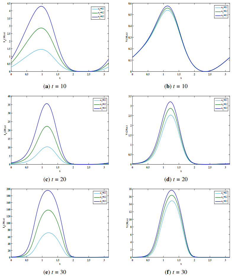
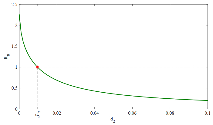
In this study, we formulate a reaction-diffusion Zika model which incorporates vector-bias, environmental transmission and spatial heterogeneity. The main question of this paper is the analysis of the threshold dynamics. For this purpose, we establish the mosquito reproduction number $R_{1}$ and basic reproduction number $R_{0}$ . Then, we analyze the dynamical behaviors in terms of $R_{1}$ and $R_{0}$ . Numerically, we find that the ignorance of the vector-bias effect will underestimate the infection risk of the Zika disease, ignorance of the spatial heterogeneity effect will overestimate the infection risk, and the environmental transmission is indispensable.

Keywords:

Citation: Liping Wang, Xinyu Wang, Dajun Liu, Xuekang Zhang, Peng Wu. Dynamical analysis of a heterogeneous spatial diffusion Zika model with vector-bias and environmental transmission[J]. Electronic Research Archive, 2024, 32(2): 1308-1332. doi: 10.3934/era.2024061

Related Papers:

[1]	Rou Lin, Min Zhao, Jinlu Zhang . Random uniform exponential attractors for non-autonomous stochastic Schrödinger lattice systems in weighted space. AIMS Mathematics, 2023, 8(2): 2871-2890. doi: 10.3934/math.2023150
[2]	Ailing Ban . Asymptotic behavior of non-autonomous stochastic Boussinesq lattice system. AIMS Mathematics, 2025, 10(1): 839-857. doi: 10.3934/math.2025040
[3]	Xin Liu . Stability of random attractors for non-autonomous stochastic $p$ -Laplacian lattice equations with random viscosity. AIMS Mathematics, 2025, 10(3): 7396-7413. doi: 10.3934/math.2025339
[4]	Xintao Li, Yunlong Gao . Random uniform attractors for fractional stochastic FitzHugh-Nagumo lattice systems. AIMS Mathematics, 2024, 9(8): 22251-22270. doi: 10.3934/math.20241083
[5]	Chunting Ji, Hui Liu, Jie Xin . Random attractors of the stochastic extended Brusselator system with a multiplicative noise. AIMS Mathematics, 2020, 5(4): 3584-3611. doi: 10.3934/math.2020233
[6]	Xintao Li, Lianbing She, Rongrui Lin . Invariant measures for stochastic FitzHugh-Nagumo delay lattice systems with long-range interactions in weighted space. AIMS Mathematics, 2024, 9(7): 18860-18896. doi: 10.3934/math.2024918
[7]	Hamood Ur Rehman, Aziz Ullah Awan, Sayed M. Eldin, Ifrah Iqbal . Study of optical stochastic solitons of Biswas-Arshed equation with multiplicative noise. AIMS Mathematics, 2023, 8(9): 21606-21621. doi: 10.3934/math.20231101
[8]	Xiaobin Yao . Random attractors for non-autonomous stochastic plate equations with multiplicative noise and nonlinear damping. AIMS Mathematics, 2020, 5(3): 2577-2607. doi: 10.3934/math.2020169
[9]	Xiao Bin Yao, Chan Yue . Asymptotic behavior of plate equations with memory driven by colored noise on unbounded domains. AIMS Mathematics, 2022, 7(10): 18497-18531. doi: 10.3934/math.20221017
[10]	Li Yang . Pullback random attractors of stochastic strongly damped wave equations with variable delays on unbounded domains. AIMS Mathematics, 2021, 6(12): 13634-13664. doi: 10.3934/math.2021793

Abstract

1. Introduction

Lattice dynamical systems arise from a variety of applications in electrical engineering, biology, chemical reaction, pattern formation and so on, see, e.g., ^{[4,7,14,19,33]}. Many researchers have discussed broadly the deterministic models in ^[6,12,34,39], etc. Stochastic lattice equations, driven by additive independent white noise, was discussed for the first time in ^[2], followed by extensions in ^{[8,13,15,16,21,23,27,32,35,36,37,38,40]}.

In this paper, we will study the long term behavior of the following second order non-autonomous stochastic lattice system driven by additive white noise: for given $\tau\in\mathbb{R}$ , $t > \tau$ and $i\in\mathbb{Z}$ ,

$\begin{equation} \begin{cases} \ddot{u}+\nu A\dot{u}+h(\dot{u})+Au+\lambda u+f(u) = g(t)+a\dot{\omega}(t),\\ u(\tau) = (u_{\tau i})_{i\in\mathbb{Z}} = u_{\tau},\; \; \dot{u}(\tau) = (u_{\tau i}^{1})_{i\in\mathbb{Z}} = u_{\tau}^{1}, \end{cases} \end{equation}$

(1.1)

where $u = (u_{i})_{i\in\mathbb{Z}}$ is a sequence in $l^{2}$ , $\nu$ and $\lambda$ are positive constants, $\dot{u} = (\dot{u}_{i})_{i\in\mathbb{Z}}$ and $\ddot{u} = (\ddot{u}_{i})_{i\in\mathbb{Z}}$ denote the fist and the second order time derivatives respectively, $Au = ((Au)_{i})_{i\in\mathbb{Z}}$ , $A\dot{u} = ((A\dot{u})_{i})_{i\in\mathbb{Z}}$ , $A$ is a linear operators defined in (2.2), $a = (a_{i})_{i\in\mathbb{ Z}}\in l^{2}$ , $f(u) = \big(f_{i}(u_{i})\big)_{i\in\mathbb{Z}}$ and $h(\dot{u}) = \big(h_{i}(\dot{u}_{i})\big)_{i\in\mathbb{Z}}$ satisfy certain conditions, $g(t) = \big(g_{i}(t)\big)_{i\in\mathbb{Z}}\in L^{2}_{loc}(\mathbb{R}, l^{2})$ is a given time dependent sequence, and $\omega(t) = W(t, \omega)$ is a two-sided real-valued Wiener process on a probability space.

The approximation we use in the paper was first proposed in ^[18,22] where the authors investigated the chaotic behavior of random equations driven by $\mathcal{G}_{\delta}(\theta_{t}\omega)$ . Since then, their work was extended by many scholars. To the best of my knowledge, there are three forms of Wong-Zakai approximations $\mathcal{G}_{\delta}(\theta_{t}\omega)$ used recenly, Euler approximation of Brownian ^{[3,10,17,20,25,28,29,30]}, Colored noise ^[5,11,26,31] and Smoothed approximation of Brownian motion by mollifiers ^[9]. In this paper, we will focus on Euler approximation of Brownian and compare the long term behavior of system (1.1) with pathwise deterministic system given by

$\begin{equation} \begin{cases} \ddot{u}^{\delta}+\nu A\dot{u}^{\delta}+h(\dot{u}^{\delta})+Au^{\delta}+\lambda u^{\delta}+f(u^{\delta}) = g(t)+a\mathcal{G}_{\delta}(\theta_{t}\omega),\\ u^{\delta}(\tau) = (u^{\delta}_{\tau i})_{i\in\mathbb{Z}} = u^{\delta}_{\tau},\; \; \dot{u}^{\delta}(\tau) = (u^{\delta,1}_{\tau i})_{i\in\mathbb{Z}} = u^{\delta,1}_{\tau}, \end{cases} \end{equation}$

(1.2)

for $\delta\in\mathbb{R}$ with $\delta\neq0$ , $\tau\in\mathbb{R}$ , $t > \tau$ and $i\in\mathbb{Z}$ , where $\mathcal{G}_{\delta}(\theta_{t}\omega)$ is defined in (3.2). Note that the solution of system (1.2) is written as $u^{\delta}$ to show its dependence on $\delta$ .

This paper is organized as follows. In Section 2, we prove the existence and uniqueness of random attractors of system (1.1). Section 3 is devoted to consider the the Wong-Zakai approximations associated with system (1.1). In Section 4, we establish the convergence of solutions and attractors for approximate system (1.2) when $\delta\rightarrow0$ .

Throughout this paper, the letter $c$ and $c_{i}(i = 1, 2, \ldots)$ are generic positive constants which may change their values from line to line.

2. Stochastic lattice system with additive white noise

In this section, we will define a continuous cocycle for second order non-autonomous stochastic lattice system (1.1), and then prove the existence and uniqueness of pullback attractors.

A standard Brownian motion or Wiener process $(W_{t})_{t\in\mathbb{R}}$ (i.e., with two-sided time) in $\mathbb{R}$ is a process with $W_{0} = 0$ and stationary independent increments satisfying $W_{t}-W_{s}\sim \mathcal{N}(0, |t-s|I)$ . $\mathcal{F}$ is the Borel $\sigma$ -algebra induced by the compact-open topology of $\Omega$ , and $P$ is the corresponding Wiener measure on $(\Omega, \mathcal{F})$ , where

$\Omega = \{\omega\in C(\mathbb{R},\mathbb{R}):\omega(0) = 0\},$

the probability space $(\Omega, \mathcal{F}, P)$ is called Wiener space. Define the time shift by

$\begin{equation} \begin{split}\nonumber \theta_{t}\omega(\cdot) = \omega(\cdot+t)-\omega(t),\quad \omega \in \Omega,\ t \in\mathbb{R}.\\ \end{split} \end{equation}$

Then $(\Omega, \mathcal{F}, P, \{\theta_{t}\}_{t\in\mathbb{R}})$ is a metric dynamical system (see ^[1]) and there exists a $\{\theta_{t}\}_{t\in\mathbb{R}}$ -invariant subset $\tilde{\Omega}\subseteq\Omega$ of full measure such that for each $\omega\in\Omega$ ,

$\begin{equation} \begin{split} \frac{\omega(t)}{t}\rightarrow0\; \; \text{as}\; \; t\rightarrow \pm\infty. \end{split} \end{equation}$

(2.1)

For the sake of convenience, we will abuse the notation slightly and write the space $\tilde{\Omega}$ as $\Omega$ .

We denote by

$l^{p} = \{u|u = (u_{i})_{i\in \mathbb{Z}},u_{i}\in \mathbb{R} ,\ \sum\limits_{i\in \mathbb{Z}}|u_{i}|^{p} < +\infty\},$

with the norm as

$\|u\|_{p}^{p} = \sum\limits_{i\in \mathbb{Z}}|u_{i}|^{p}.$

In particular, $l^{2}$ is a Hilbert space with the inner product $(\cdot, \cdot)$ and norm $\|\cdot\|$ given by

$(u,v) = \sum\limits_{i\in \mathbb{Z}}u_{i}v_{i},\qquad \|u\|^{2} = \sum\limits_{i\in \mathbb{Z}}|u_{i}|^{2},$

for any $u = (u_{i})_{i\in \mathbb{Z}}, \ v = (v_{i})_{i\in \mathbb{Z}}\in l^{2}$ .

Define linear operators $B$ , $B^{*}$ , and $A$ acting on $l^{2}$ in the following way: for any $u = (u_{i})_{i\in\mathbb{Z}}\in l^{2}$ ,

$(Bu)_{i} = u_{i+1}-u_{i},\qquad(B^{*}u)_{i} = u_{i-1}-u_{i},$

and

$\begin{equation} \begin{split} (Au)_{i} = 2u_{i}-u_{i+1}-u_{i-1}. \end{split} \end{equation}$

(2.2)

Then we find that $A = BB^{*} = B^{*}B$ and $(B^{*}u, v) = (u, Bv)$ for all $u, v\in l^{2}$ .

Also, we let $F_{i}(s) = \int_{0}^{s}f_{i}(r)dr$ , $h(\dot{u}) = (h_{i}(\dot{u}_{i}))_{i\in\mathbb{Z}}$ , $f(u) = (f_{i}(u_{i}))_{i\in\mathbb{Z}}$ with $f_{i}, h_{i}\in C^{1}(\mathbb{R}, \mathbb{R})$ satisfy the following assumptions:

$\begin{equation} |f_{i}(s)|\leq \alpha_{1}(|s|^{p}+|s|), \end{equation}$

(2.3)

$\begin{equation} sf_{i}(s)\geq \alpha_{2}F_{i}(s)\geq\alpha_{3}|s|^{p+1}, \end{equation}$

(2.4)

and

$\begin{equation} h_{i}(0) = 0,\; \; 0 < h_{1}\leq h_{i}'(s)\leq h_{2},\; \; \forall s\in\mathbb{R}, \end{equation}$

(2.5)

where $p > 1$ , $\alpha_{i}$ and $h_{j}$ are positive constants for $i = 1, 2, 3$ and $j = 1, 2$ .

In addition, we let

$\begin{equation} \begin{split} \beta = \frac{h_{1}\lambda}{4\lambda+h_{2}^{2}},\; \; \beta < \frac{1}{\nu}, \end{split} \end{equation}$

(2.6)

and

$\begin{equation} \begin{split} \sigma = \frac{h_{1}\lambda}{\sqrt{4\lambda+h_{2}^{2}}(h_{2}+\sqrt{4\lambda+h_{2}^{2}})}. \end{split} \end{equation}$

(2.7)

For any $u, v\in l^{2}$ , we define a new inner product and norm on $l^{2}$ by

$(u,v)_{\lambda} = (1-\nu\beta)(Bu,Bv)+\lambda(u,v),\; \; \|u\|^{2}_{\lambda} = (u,u)_{\lambda} = (1-\nu\beta)\|Bu\|^{2}+\lambda\|u\|^{2}.$

Denote

$l^{2} = (l^{2},(\cdot,\cdot),\|\cdot\|),\qquad l^{2}_{\lambda} = (l^{2},(\cdot,\cdot)_{\lambda},\|\cdot\|_{\lambda}).$

Then the norms $\|\cdot\|$ and $\|\cdot\|_{\lambda}$ are equivalent to each other.

Let $E = l^{2}_{\lambda}\times l^{2}$ endowed with the inner product and norm

$(\psi_{1},\psi_{2})_{E} = (u^{(1)},u^{(2)})_{\lambda}+(v^{(1)},v^{(2)}),\qquad \|\psi\|_{E}^{2} = \|u\|^{2}_{\lambda}+\|v\|^{2},$

for $\psi_{j} = (u^{(j)}, v^{(j)})^{T} = \big((u^{(j)}_{i}), (v^{(j)}_{i})\big)^{T}_{i\in \mathbb{Z}}\in E, \ j = 1, 2, \quad \psi = (u, v)^{T} = \big((u_{i}), (v_{i})\big)^{T}_{i\in \mathbb{Z}}\in E.$

A family $D = \{D(\tau, \omega):\tau\in\mathbb{R}, \omega\in\Omega\}$ of bounded nonempty subsets of $E$ is called tempered (or subexponentially growing) if for every $\epsilon > 0$ , the following holds:

$\lim\limits_{t\rightarrow -\infty}e^{\epsilon t}\|D(\tau+t,\theta_{t}\omega)\|^{2} = 0,$

where $\|D\| = \mathop{\sup}\limits_{x\in D}\|x\|_{E}$ . In the sequel, we denote by $\mathcal{D}$ the collection of all families of tempered nonempty subsets of $E$ , i.e.,

$\begin{equation} \nonumber \mathcal{D} = \{D = \{D(\tau,\omega):\tau\in\mathbb{R},\omega\in\Omega\}:D\; \text{is tempered in}\; E\}. \end{equation}$

The following conditions will be needed for $g$ when deriving uniform estimates of solutions, for every $\tau\in\mathbb{R}$ ,

$\begin{equation} \int_{-\infty}^{\tau}e^{\gamma s}\|g(s)\|^{2}ds < \infty, \end{equation}$

(2.8)

and for any $\varsigma > 0$

$\begin{equation} \lim\limits_{t\rightarrow -\infty}e^{\varsigma t}\int_{-\infty}^{0}e^{ \gamma s}\|g(s+t)\|^{2}ds = 0, \end{equation}$

(2.9)

where $\gamma = \min\{\frac{\sigma}{2}, \frac{\alpha_{2}\beta}{p+1}\}$ .

Let $\bar{v} = \dot{u}+\beta u$ and $\bar{\varphi} = (u, \bar{v})^{T}$ , then system (1.1) can be rewritten as

$\begin{eqnarray} \dot{\bar{\varphi}}+L_{1}(\bar{\varphi}) = H_{1}(\bar{\varphi})+G_{1}(\omega), \end{eqnarray}$

(2.10)

with initial conditions

$\bar{\varphi}_{\tau} = (u_{\tau},\bar{v}_{\tau})^{T} = (u_{\tau},u_{\tau}^{1}+\beta u_{\tau})^{T},$

where

$L_{1}(\bar{\varphi}) = \left( \begin{array}{ccc} \beta u-\bar{v} \\ (1-\nu\beta)Au+\nu A\bar{v}+\lambda u +\beta^{2} u-\beta\bar{v} \end{array} \right) + \left( \begin{array}{ccc} 0 \\ h(\bar{v}-\beta u) \end{array} \right) ,$

$H_{1}(\bar{\varphi}) = \left( \begin{array}{ccc} 0 \\ -f(u)+g(t) \end{array} \right),\; \; \; \; G_{1}(\omega) = \left( \begin{array}{ccc} 0 \\ a\dot\omega(t) \end{array} \right) .$

Denote

$v(t) = \bar{v}(t)-a\omega(t) \; \; \text{and}\; \; \varphi = (u,v)^{T}.$

By (2.10) we have

$\begin{eqnarray} \dot{\varphi}+L(\varphi) = H(\varphi)+G(\omega), \end{eqnarray}$

(2.11)

with initial conditions

$\varphi_{\tau} = (u_{\tau},v_{\tau})^{T} = (u_{\tau},u_{\tau}^{1}+\beta u_{\tau}-a\omega(\tau))^{T},$

where

$L(\varphi) = \left( \begin{array}{ccc} \beta u-v \\ (1-\nu\beta) Au+\nu Av+\lambda u+\beta^{2} u-\beta v \end{array} \right) + \left( \begin{array}{ccc} 0 \\ h(v-\beta u+a\omega(t)) \end{array} \right) ,$

$H(\varphi) = \left( \begin{array}{ccc} 0 \\ -f(u)+g(t) \end{array} \right),\; \; \; \; G(\omega) = \left( \begin{array}{ccc} a\omega(t)\\ \beta a\omega(t)-\nu Aa\omega(t) \end{array} \right) .$

Note that system (2.11) is a deterministic functional equation and the nonlinearity in (2.11) is locally Lipschitz continuous from $E$ to $E$ . Therefore, by the standard theory of functional differential equations, system (2.11) is well-posed. Thus, we can define a continuous cocycle $\Phi_{0}:\mathbb{R}^{+}\times\mathbb{R}\times \Omega\times E\rightarrow E$ associated with system (2.10), where for $\tau\in\mathbb{R}$ , $t\in\mathbb{R}^{+}$ and $\omega\in\Omega$

$\begin{equation} \begin{split}\nonumber \Phi_{0}(t,\tau,\omega,\bar{\varphi}_{\tau})& = \bar{\varphi}(t+\tau,\tau,\theta_{-\tau}\omega,\bar{\varphi}_{\tau})\\ & = (u(t+\tau,\tau,\theta_{-\tau}\omega,u_{\tau}),\bar{v}(t+\tau,\tau,\theta_{-\tau}\omega,\bar{v}_{\tau}))^{T}\\ & = (u(t+\tau,\tau,\theta_{-\tau}\omega,u_{\tau}),v(t+\tau,\tau,\theta_{-\tau}\omega,v_{\tau})+a(\omega(t)-\omega(-\tau)))^{T}\\ & = \varphi(t+\tau,\tau,\theta_{-\tau}\omega,\varphi_{\tau})+(0,a(\omega(t)-\omega(-\tau)))^{T}, \end{split} \end{equation}$

where $v_{\tau} = \bar{v}_{\tau}+a\omega(-\tau)$ .

Lemma 2.1. Suppose that (2.3)–(2.8) hold. Then for every $\tau\in\mathbb{R}$ , $\omega\in\Omega$ , and $T > 0$ , there exists $c = c(\tau, \omega, T) > 0$ such that for all $t\in[\tau, \tau+T]$ , the solution $\varphi$ of system (2.11) satisfies

$\begin{equation} \begin{split}\nonumber \|\varphi(t,\tau,\omega,\varphi_{\tau})\|^{2}_{E} +\int_{\tau}^{t}\|\varphi(s,\tau,\omega,\varphi_{\tau})\|^{2}_{E}ds \leq& c\int^{t}_{\tau}\big(\|g(s)\|^{2}+|\omega(s)|^{2}+| \omega(s)|^{p+1}\big)ds\\ &+c\big(\|\varphi_{\tau}\|^{2}_{E}+2\sum\limits_{i\in\mathbb{Z}} F_{i}(u_{\tau,i})\big). \end{split} \end{equation}$

Proof. Taking the inner product $(\cdot, \cdot)_{E}$ on both side of the system (2.11) with $\varphi$ , it follows that

$\begin{equation} \begin{split} &\frac{1}{2}\frac{d}{dt}\|\varphi\|^{2}_{E}+(L(\varphi),\varphi)_{E} = (H(\varphi),\varphi)_{E}+(G(\omega),\varphi)_{E}. \end{split} \end{equation}$

(2.12)

For the second term on the left-hand side of (2.12), we have

$\begin{equation} \begin{split}\nonumber (L(\varphi),\varphi)_{E} = \beta\|u\|^{2}_{\lambda}+\beta^{2}(u,v)-\beta\|v\|^{2}+\nu(Av,v)+(h(v-\beta u+a\omega(t)),v). \end{split} \end{equation}$

By the mean value theorem and (2.5), there exists $\xi_{i}\in(0, 1)$ such that

$\begin{equation} \begin{split}\nonumber &\beta^{2}(u,v)+(h(v-\beta u+a\omega(t)),v)\\ & = \beta^{2}(u,v) +\sum\limits_{i\in\mathbb{Z}}h'_{i}(\xi_{i}(v_{i}-\beta u_{i}+a_{i}\omega(t)))(v_{i}-\beta u_{i}+a_{i}\omega(t))v_{i}\\ &\geq (\beta^{2}-h_{2}\beta)\|u\|\|v\|+h_{1}\|v\|^{2}-h_{2}|(a\omega(t),v)|. \end{split} \end{equation}$

Then

$\begin{equation} \begin{split}\nonumber (L(\varphi),\varphi)_{E}-\sigma\|\varphi\|^{2}_{E}-\frac{h_{1}}{2}\|v\|^{2} \geq &(\beta-\sigma)\|u\|^{2}_{\lambda}+(\frac{h_{1}}{2}-\beta-\sigma)\|v\|^{2}\\&- \frac{\beta h_{2}}{\sqrt{\lambda}}\|u\|_{\lambda}\|v\|-h_{2}|(a\omega(t),v)|, \end{split} \end{equation}$

which along with (2.6) and (2.7) implies that

$\begin{equation} \begin{split} (L(\varphi),\varphi)_{E}\geq\sigma\|\varphi\|^{2}_{E}+\frac{h_{1}}{2}\|v\|^{2} -\frac{\sigma+h_{1}}{6}\|v\|^{2}-c|\omega(t)|^{2}\|a\|^{2}. \end{split} \end{equation}$

(2.13)

As to the first term on the right-hand side of (2.12), by (2.3) and (2.4) we get

$\begin{equation} \begin{split} (H(\varphi),\varphi)_{E}& = (-f(u),\dot{u}+\beta u-a\omega(t))+(g(t),v)\\ &\leq-\frac{d}{dt}\big(\sum\limits_{i\in\mathbb{Z}}F_{i}(u_{i})\big)-\alpha_{2}\beta\sum\limits_{i\in\mathbb{Z}}F_{i}(u_{i}) +\alpha_{1}\sum\limits_{i\in\mathbb{Z}}(|u_{i}|^{p}+|u_{i}|)|a_{i}\omega(t)|+(g(t),v)\\ &\leq-\frac{d}{dt}\big(\sum\limits_{i\in\mathbb{Z}}F_{i}(u_{i})\big)-\frac{\alpha_{2}\beta}{p+1}\sum\limits_{i\in\mathbb{Z}}F_{i}(u_{i}) +c|\omega(t)|^{p+1}\|a\|^{p+1}\\ &\quad+\frac{\sigma\lambda}{4}\|u\|^{2}+c\|a\|^{2}|\omega(t)|^{2}+\frac{\sigma+h_{1}}{6}\|v\|^{2}+c\|g(t)\|^{2}. \end{split} \end{equation}$

(2.14)

The last term of (2.12) is bounded by

$\begin{equation} \begin{split} (G(\omega),\varphi)_{E}& = \omega(t)(a,u)_{\lambda}+\beta \omega(t)(a,v)-\nu\omega(t)(Aa,v)\\ &\leq \frac{\sigma}{4}\|u\|^{2}_{\lambda}+\frac{1}{\sigma}\|a\|^{2}_{\lambda}|\omega(t)|^{2}+\frac{\sigma+h_{1}}{6}\|v\|^{2}+c|\omega(t)|^{2}\|a\|^{2}. \end{split} \end{equation}$

(2.15)

It follows from (2.12)–(2.15) that

$\begin{equation} \begin{split} &\frac{d}{dt}\Big(\|\varphi\|_{E}^{2}+2\sum\limits_{i\in\mathbb{Z}} F_{i}(u_{i})\Big) +\gamma\Big(\|\varphi\|_{E}^{2}+2\sum\limits_{i\in\mathbb{Z}} F_{i}(u_{i})\Big)+\gamma\|\varphi\|_{E}^{2}\\ &\leq c\Big(\|g(t)\|^{2}+|\omega(t)|^{2}+|\omega(t)|^{p+1}\Big), \end{split} \end{equation}$

(2.16)

where $\gamma = \min\{\frac{\sigma}{2}, \frac{\alpha_{2}\beta}{p+1}\}$ . Multiplying (2.16) by $e^{\gamma t}$ and then integrating over $(\tau, t)$ with $t\geq\tau$ , we get for every $\omega\in\Omega$

$\begin{equation} \begin{split} &\|\varphi(t,\tau,\omega,\varphi_{\tau})\|_{E}^{2} +\gamma\int^{t}_{\tau}e^{\gamma(s-t)}\|\varphi(s,\tau,\omega,\varphi_{\tau})\|_{E}^{2}ds\\ &\leq e^{\gamma(\tau-t)}\Big(\|\varphi_{\tau}\|_{E}^{2}+2\sum\limits_{i\in\mathbb{Z}} F_{i}(u_{\tau,i})\Big)+c\int^{t}_{\tau}e^{\gamma(s-t)}\Big(\|g(s)\|^{2}+|\omega(s)|^{2}+|\omega(s)|^{p+1}\Big)ds, \end{split} \end{equation}$

(2.17)

which implies desired result.

Lemma 2.2. Suppose that (2.3)–(2.9) hold. Then the continuous cocycle $\Phi_{0}$ associated with system (2.10) has a closed measurable $\mathcal{D}$ -pullback absorbing set $K_{0} = \{K_{0}(\tau, \omega):\tau\in\mathbb{R}, \omega\in\Omega\}\in\mathcal{D}$ , where for every $\tau\in\mathbb{R}$ and $\omega\in\Omega$

$\begin{equation} \begin{split} K_{0}(\tau,\omega) = \{\bar{\varphi}\in E:\|\bar{\varphi}\|^{2}_{E}\leq R_{0}(\tau,\omega)\}, \end{split} \end{equation}$

(2.18)

where $\bar{\varphi}_{\tau-t}\in D(\tau-t, \theta_{-t}\omega)$ and $R_{0}(\tau, \omega)$ is given by

$\begin{equation} \begin{split} R_{0}(\tau,\omega) = c+c|\omega(-\tau)|^{2}+c\int^{0}_{-\infty}e^{\gamma s}\Big(\|g(s+\tau)\|^{2}+|\omega(s)-\omega(-\tau)|^{2}+| \omega(s)-\omega(-\tau)|^{p+1}\Big)ds, \end{split} \end{equation}$

(2.19)

where $c$ is a positive constant independent of $\tau$ , $\omega$ and $\mathcal{D}$ .

Proof. By (2.17), we get for every $\tau\in\mathbb{R}$ , $t\in\mathbb{R}^{+}$ and $\omega\in\Omega$

$\begin{equation} \begin{split} &\|\varphi(\tau,\tau-t,\theta_{-\tau}\omega,\varphi_{\tau-t})\|^{2}_{E}+\gamma\int_{\tau-t}^{\tau}e^{\gamma(s-\tau)}\|\varphi(s,\tau-t,\theta_{-\tau}\omega,\varphi_{\tau-t})\|^{2}_{E}ds\\ &\leq e^{-\gamma t}\Big(\|\varphi_{\tau-t}\|^{2}_{E}+2\sum\limits_{i\in\mathbb{Z}} F_{i}(u_{\tau-t,i})\Big)\\ &\quad +c\int^{\tau}_{\tau-t}e^{\gamma(s-\tau)}\Big(\|g(s)\|^{2}+|\omega(s-\tau)-\omega(-\tau)|^{2}+|\omega(s-\tau)-\omega(-\tau)|^{p+1}\Big)ds\\ &\leq e^{-\gamma t}\Big(\|\varphi_{\tau-t}\|^{2}_{E}+2\sum\limits_{i\in\mathbb{Z}} F_{i}(u_{\tau-t,i})\Big)\\ &\quad +c\int^{0}_{-t}e^{\gamma s}\Big(\|g(s+\tau)\|^{2}+|\omega(s)-\omega(-\tau)|^{2}+| \omega(s)-\omega(-\tau)|^{p+1}\Big)ds. \end{split} \end{equation}$

(2.20)

By (2.1) and (2.8), the last integral on the right-hand side of (2.20) is well defined. For any $s\geq \tau-t$ ,

$\begin{equation} \begin{split}\nonumber &\bar{\varphi}(s,\tau-t,\theta_{-\tau}\omega,\bar{\varphi}_{\tau-t}) = \varphi(s,\tau-t,\theta_{-\tau}\omega,\varphi_{\tau-t})+(0,a(\omega(s-\tau)-\omega(-\tau)))^{T}, \end{split} \end{equation}$

which along with (2.20) implies that

$\begin{equation} \begin{split} &\|\bar{\varphi}(\tau,\tau-t,\theta_{-\tau}\omega,\bar{\varphi}_{\tau-t})\|^{2}_{E} +\gamma\int_{\tau-t}^{\tau}e^{\gamma(s-\tau)}\|\bar{\varphi}(s,\tau-t,\theta_{-\tau}\omega,\bar{\varphi}_{\tau-t})\|^{2}_{E}ds\\ &\leq2\|\varphi(\tau,\tau-t,\theta_{-\tau}\omega,\varphi_{\tau-t})\|^{2}_{E} +2\gamma\int_{\tau-t}^{\tau}e^{\gamma(s-\tau)}\|\varphi(s,\tau-t,\theta_{-\tau}\omega,\varphi_{\tau-t})\|^{2}_{E}ds\\ &\quad+2\|a\|^{2}\Big(|\omega(-\tau)|^{2}+\gamma\int_{\tau-t}^{\tau}e^{\gamma(s-\tau)}|\omega(s-\tau)-\omega(-\tau)|^{2}ds\Big)\\ &\leq 4e^{-\gamma t}\Big(\|\bar{\varphi}_{\tau-t}\|^{2}_{E}+\|a\|^{2}|\omega(-t)-\omega(-\tau)|^{2}+\sum\limits_{i\in\mathbb{Z}} F_{i}(u_{\tau-t,i})\Big)+c|\omega(-\tau)|^{2}\\ &\quad +c\int^{0}_{-\infty}e^{\gamma s}\Big(\|g(s+\tau)\|^{2}+|\omega(s)-\omega(-\tau)|^{2}+| \omega(s)-\omega(-\tau)|^{p+1}\Big)ds.\\ \end{split} \end{equation}$

(2.21)

By (2.3) and (2.4) we have

$\begin{equation} \begin{split} \sum\limits_{i\in\mathbb{Z}} F_{i}(u_{\tau-t,i})\leq \frac{1}{\alpha_{2}}\sum\limits_{i\in\mathbb{Z}} f_{i}(u_{\tau-t,i})u_{\tau-t, i} \leq\frac{1}{\alpha_{2}}\max\limits_{-\|u_{\tau-t}\|\leq s\leq\|u_{\tau-t}\|}|f'_{i}(s)|\|u_{\tau-t}\|^{2}. \end{split} \end{equation}$

(2.22)

Using $\bar{\varphi}_{\tau-t}\in D(\tau-t, \theta_{-t}\omega)$ , (2.1) and (2.22), we find

$\begin{equation} \begin{split} \limsup\limits_{t\rightarrow +\infty}4e^{-\gamma t}\Big(\|\bar{\varphi}_{\tau-t}\|^{2}_{E}+\|a\|^{2}|\omega(-t)-\omega(-\tau)|^{2}+\sum\limits_{i\in\mathbb{Z}} F_{i}(u_{\tau-t,i})\Big) = 0, \end{split} \end{equation}$

(2.23)

which along with (2.21) implies that there exists $T = T(\tau, \omega, D) > 0$ such that for all $t\geq T$ ,

(2.24)

where $c$ is a positive constant independent of $\tau$ , $\omega$ and $D$ . Note that $K_{0}$ given by (2.18) is closed measurable random set in $E$ . Given $\tau\in\mathbb{R}$ , $\omega\in\Omega$ , and $D\in\mathcal{D}$ , it follows from (2.24) that for all $t\geq T$ ,

$\begin{equation} \begin{split} \Phi_{0}(t,\tau-t,\theta_{-t}\omega,D(\tau-t,\theta_{-t}\omega))\subseteq K_{0}(\tau,\omega), \end{split} \end{equation}$

(2.25)

which implies that $K_{0}$ pullback attracts all elements in $\mathcal{D}$ . By (2.1) and (2.9), one can easily check that $K_{0}$ is tempered, which along with (2.25) completes the proof.

Next, we will get uniform estimates on the tails of solutions of system (2.10).

Lemma 2.3. Suppose that (2.3)–(2.9) hold. Then for every $\tau\in\mathbb{R}$ , $\omega\in\Omega$ , $D = \{D(\tau, \omega):\tau\in\mathbb{R}, \omega\in\Omega\}\in\mathcal{D}$ and $\varepsilon > 0$ , there exist $T = T(\tau, \omega, D, \varepsilon) > 0$ and $N = N(\tau, \omega, \varepsilon) > 0$ such that for all $t\geq T$ , the solution $\bar{\varphi}$ of system (2.10) satisfies

$\begin{equation} \begin{split}\nonumber \sum\limits_{|i|\geq N}|\bar{\varphi}_{i}(\tau,\tau-t,\theta_{-\tau}\omega,\bar{\varphi}_{\tau-t,i})|_{E}^{2}\leq\varepsilon,\\ \end{split} \end{equation}$

where $\bar{\varphi}_{\tau-t}\in D(\tau-t, \theta_{-t}\omega)$ and $|\bar{\varphi}_{i}|_{E}^{2} = (1-\nu\beta)|Bu|_{i}^{2}+\lambda |u_{i}|^{2}+|\bar{v}_{i}|^{2}$ .

Proof. Let $\eta$ be a smooth function defined on $\mathbb{R}^{+}$ such that $0\leq\eta(s)\leq1$ for all $s\in\mathbb{R}^{+}$ , and

$\begin{equation} \nonumber \eta(s) = \left\{\begin{array}{l} 0,\; \; 0\leq s\leq1;\\ 1,\; \; s\geq2. \end{array}\right. \end{equation}$

Then there exists a constant $C_{0}$ such that $|\eta'(s)|\leq C_{0}$ for $s\in\mathbb{R}^{+}$ . Let $k$ be a fixed positive integer which will be specified later, and set $x = (x_{i})_{i\in\mathbb{Z}}$ , $y = (y_{i})_{i\in\mathbb{Z}}$ with $x_{i} = \eta(\frac{|i|}{k})u_{i}$ , $y_{i} = \eta(\frac{|i|}{k})v_{i}$ . Note $\psi = (x, y)^{T} = ((x_{i}), (y_{i}))^{T}_{i\in\mathbb{Z}}$ . Taking the inner product of system (2.11) with $\psi$ , we have

$\begin{equation} \begin{split} (\dot{\varphi},\psi)_{E}+(L(\varphi),\psi)_{E} = (H(\varphi),\psi)_{E}+(G,\psi)_{E}. \end{split} \end{equation}$

(2.26)

For the first term of (2.26), we have

$\begin{equation} \begin{split} (\dot{\varphi},\psi)_{E}& = (1-\nu\beta)\sum\limits_{i\in\mathbb{Z}}(B\dot{u})_{i}(Bx)_{i}+\lambda\sum\limits_{i\in\mathbb{Z}}\dot{u}_{i}x_{i} +\sum\limits_{i\in\mathbb{Z}}\dot{v}_{i}y_{i}\\ & = \frac{1}{2}\frac{d}{dt}\sum\limits_{i\in\mathbb{Z}}\eta(\frac{|i|}{k})|\varphi_{i}|^{2}_{E} +(1-\nu\beta)\sum\limits_{i\in\mathbb{Z}}(B\dot{u})_{i}\Big((Bx)_{i}-\eta(\frac{|i|}{k})(Bu)_{i}\Big)\\ &\geq\frac{1}{2}\frac{d}{dt}\sum\limits_{i\in\mathbb{Z}}\eta(\frac{|i|}{k})|\varphi_{i}|^{2}_{E} -\frac{(1-\nu\beta)C_{0}}{k}\sum\limits_{i\in\mathbb{Z}}|(B(v-\beta u+a\omega(t))_{i}||u_{i+1}|\\ &\geq\frac{1}{2}\frac{d}{dt}\sum\limits_{i\in\mathbb{Z}}\eta(\frac{|i|}{k})|\varphi_{i}|^{2}_{E} -\frac{c}{k}\|\varphi\|^{2}_{E}-\frac{c}{k}|\omega(t)|^{2}\|a\|^{2}, \end{split} \end{equation}$

(2.27)

where $|\varphi_{i}|_{E}^{2} = (1-\nu\beta)|Bu|_{i}^{2}+\lambda |u_{i}|^{2}+|v_{i}|^{2}$ . As to the second term on the left-hand side of (2.26), we get

$\begin{equation} \begin{split}\nonumber (L(\varphi),\psi)_{E} = &\beta(1-\nu\beta)(Au,x)+(1-\nu\beta)((Au,y)-(Av,x))+\nu(Av,y)+\lambda\beta(u,x)\\ &+\beta^{2}(u,y)-\beta(v,y)+(h(v-\beta u+a\omega(t)),y). \end{split} \end{equation}$

It is easy to check that

$\begin{equation} \begin{split}\nonumber (Au,x) = \sum\limits_{i\in\mathbb{Z}}(Bu)_{i}\Big(\eta(\frac{|i|}{k})(Bu)_{i}+(Bx)_{i}-\eta(\frac{|i|}{k})(Bu)_{i}\Big) \geq\sum\limits_{i\in\mathbb{Z}}\eta(\frac{|i|}{k})|Bu|_{i}^{2}-\frac{2C_{0}}{k}\|u\|^{2}, \end{split} \end{equation}$

$\begin{equation} \begin{split}\nonumber (Av,y) = \sum\limits_{i\in\mathbb{Z}}(Bv)_{i}\Big(\eta(\frac{|i|}{k})(Bv)_{i}+(By)_{i}-\eta(\frac{|i|}{k})(Bv)_{i}\Big) \geq\sum\limits_{i\in\mathbb{Z}}\eta(\frac{|i|}{k})|Bv|_{i}^{2}-\frac{2C_{0}}{k}\|v\|^{2}, \end{split} \end{equation}$

and

$\begin{equation} \begin{split}\nonumber (Au,y)-(Av,x)\geq-\frac{C_{0}}{k}\sum\limits_{i\in\mathbb{Z}}|(Bu)_{i}||v_{i+1}|-\frac{C_{0}}{k}\sum\limits_{i\in\mathbb{Z}}|(Bv)_{i}||u_{i+1}| \geq-\frac{2 C_{0}}{k}(\|u\|^{2}+\|v\|^{2}). \end{split} \end{equation}$

By the mean value theorem and (2.5), there exists $\xi_{i}\in(0, 1)$ such that

$\begin{equation} \begin{split}\nonumber &\beta^{2}(u,y)+(h(v-\beta u+a\omega(t)),y)\\ & = \beta^{2}\sum\limits_{i\in\mathbb{Z}}\eta(\frac{|i|}{k})u_{i}v_{i} +\sum\limits_{i\in\mathbb{Z}}h'_{i}(\xi_{i}(v_{i}-\beta u_{i}+a_{i}\omega(t)))(v_{i}-\beta u_{i}+a_{i}\omega(t))\eta(\frac{|i|}{k})v_{i}\\ &\geq \beta(\beta-h_{2})\sum\limits_{i\in\mathbb{Z}}\eta(\frac{|i|}{k})|u_{i}v_{i}|+h_{1}\sum\limits_{i\in\mathbb{Z}}\eta(\frac{|i|}{k})|v_{i}|^{2} -h_{2}\sum\limits_{i\in\mathbb{Z}}\eta(\frac{|i|}{k})|v_{i}a_{i}\omega(t)|. \end{split} \end{equation}$

Then

$\begin{equation} \begin{split}\nonumber &(L(\varphi),\varphi)_{E}-\sigma\sum\limits_{i\in\mathbb{Z}}\eta(\frac{|i|}{k})|\varphi_{i}|^{2}_{E} -\frac{h_{1}}{2}\sum\limits_{i\in\mathbb{Z}}\eta(\frac{|i|}{k})|v_{i}|^{2}\\ &\geq (\beta-\sigma)\sum\limits_{i\in\mathbb{Z}}\eta(\frac{|i|}{k})\Big((1-\nu\beta)|Bu|_{i}^{2}+\lambda u_{i}^{2}\Big)+(\frac{h_{1}}{2}-\beta-\sigma)\sum\limits_{i\in\mathbb{Z}}\eta(\frac{|i|}{k})|v_{i}|^{2}\\ &\quad-\frac{\beta h_{2}}{\sqrt{\lambda}}\sum\limits_{i\in\mathbb{Z}}\eta(\frac{|i|}{k})|v_{i}|\Big((1-\nu\beta)(Bu)_{i}^{2}+\lambda| u_{i}|^{2}\Big)^{\frac{1}{2}}-h_{2}\sum\limits_{i\in\mathbb{Z}}\eta(\frac{|i|}{k})|v_{i}a_{i}\omega(t)|-\frac{c}{k}\|\varphi\|^{2}_{E}, \end{split} \end{equation}$

which along with (2.6) and (2.7) implies that

$\begin{equation} \begin{split} (L(\varphi),\varphi)_{E}&\geq\sigma\sum\limits_{i\in\mathbb{Z}}\eta(\frac{|i|}{k})|\varphi_{i}|^{2}_{E}+ \frac{h_{1}}{2}\sum\limits_{i\in\mathbb{Z}}\eta(\frac{|i|}{k})|v_{i}|^{2}-\frac{c}{k}\|\varphi\|^{2}_{E}-h_{2}\sum\limits_{i\in\mathbb{Z}}\eta(\frac{|i|}{k})|v_{i}a_{i}\omega(t)|\\ &\geq\sigma\sum\limits_{i\in\mathbb{Z}}\eta(\frac{|i|}{k})|\varphi_{i}|^{2}_{E}+ \frac{h_{1}}{6}\sum\limits_{i\in\mathbb{Z}}\eta(\frac{|i|}{k})|v_{i}|^{2}-\frac{c}{k}\|\varphi\|^{2}_{E} -c\sum\limits_{i\in\mathbb{Z}}\eta(\frac{|i|}{k})|a_{i}|^{2}|\omega(t)|^{2}. \end{split} \end{equation}$

(2.28)

As to the first term on the right-hand side of (2.26), by (2.3) and (2.4)we get

$\begin{equation} \begin{split} (H(\varphi),\psi)_{E}& = -\sum\limits_{i\in\mathbb{Z}}\eta(\frac{|i|}{k})f_{i}(u_{i})(\dot{u_{i}}+\beta u_{i}-a_{i}\omega(t))+\sum\limits_{i\in\mathbb{Z}}\eta(\frac{|i|}{k})g_{i}(t)v_{i}\\ &\leq-\frac{d}{dt}\big(\sum\limits_{i\in\mathbb{Z}}\eta(\frac{|i|}{k})F_{i}(u_{i})\big) -\frac{\alpha_{2}\beta}{p+1}\sum\limits_{i\in\mathbb{Z}}\eta(\frac{|i|}{k})F_{i}(u_{i})\\ &\quad+c\sum\limits_{i\in\mathbb{Z}}\eta(\frac{|i|}{k})|\omega(t)|^{p+1}|a_{i}|^{p+1} +\frac{\sigma\lambda}{4}\sum\limits_{i\in\mathbb{Z}}\eta(\frac{|i|}{k})|u_{i}|^{2}\\ &\quad+c\sum\limits_{i\in\mathbb{Z}}\eta(\frac{|i|}{k})|a_{i}|^{2}|\omega(t)|^{2} +\frac{\sigma}{6} \sum\limits_{i\in\mathbb{Z}}\eta(\frac{|i|}{k})|v_{i}|^{2} +c\sum\limits_{i\in\mathbb{Z}}\eta(\frac{|i|}{k})|g_{i}(t)|^{2}. \end{split} \end{equation}$

(2.29)

For the last term of (2.26), we have

$\begin{equation} \begin{split} (G,\psi)_{E}& = \omega(t)(a,x)_{\lambda}+\beta \omega(t)(a,y)-\nu\omega(t)(Aa,y)\\ & = \omega(t)(1-\nu\beta)(Ba,Bx)-\nu\omega(t)(Ba,By)+\lambda\omega(t)(a,x)+\beta \omega(t)(a,y), \end{split} \end{equation}$

(2.30)

As to the first two terms on the right-hand side of (2.30), we get

$\begin{equation} \begin{split} \omega(t)(1-\nu\beta)(Ba,Bx)& = \omega(t)(1-\nu\beta)\sum\limits_{i\in\mathbb{Z}}(a_{i+1}-a_{i})\Big(\eta(\frac{|i+1|}{k})u_{i+1}-\eta(\frac{|i|}{k})u_{i}\Big)\\ &\leq\Big(\sum\limits_{i\in\mathbb{Z}}\eta(\frac{|i+1|}{k})u_{i+1}^{2}\Big)^{\frac{1}{2}}\Big(\sum\limits_{i\in\mathbb{Z}}\eta(\frac{|i+1|}{k})\big(\omega(t)(1-\nu\beta)(a_{i+1}-a_{i})\big)^{2}\Big)^{\frac{1}{2}}\\ &\quad+\Big(\sum\limits_{i\in\mathbb{Z}}\eta(\frac{|i|}{k})u_{i}^{2}\Big)^{\frac{1}{2}}\Big(\sum\limits_{i\in\mathbb{Z}}\eta(\frac{|i|}{k})\big(\omega(t)(1-\nu\beta)(a_{i+1}-a_{i})\big)^{2}\Big)^{\frac{1}{2}}\\ &\leq \frac{\sigma\lambda}{8}\sum\limits_{i\in\mathbb{Z}}\eta(\frac{|i|}{k})u_{i}^{2}+c|\omega(t)|^{2}\sum\limits_{|i|\geq k}a_{i}^{2}, \end{split} \end{equation}$

(2.31)

and

$\begin{equation} \begin{split} -\nu\omega(t)(Ba,By)& = -\nu\omega(t)\sum\limits_{i\in\mathbb{Z}}(a_{i+1}-a_{i})\Big(\eta(\frac{|i+1|}{k})v_{i+1}-\eta(\frac{|i|}{k})v_{i}\Big)\\ &\leq \frac{\sigma}{6}\sum\limits_{i\in\mathbb{Z}}\eta(\frac{|i|}{k})v_{i}^{2}+c|\omega(t)|^{2}\sum\limits_{|i|\geq k}a_{i}^{2}. \end{split} \end{equation}$

(2.32)

The last two terms of (2.30) is bounded by

$\begin{equation} \begin{split} \lambda\omega(t)(a,x)+\beta \omega(t)(a,y)\leq \frac{\sigma\lambda}{8}\sum\limits_{i\in\mathbb{Z}}\eta(\frac{|i|}{k})u_{i}^{2}+\frac{\sigma+h_{1}}{6}\sum\limits_{i\in\mathbb{Z}}\eta(\frac{|i|}{k})v_{i}^{2} +c|\omega(t)|^{2}\sum\limits_{|i|\geq k}a_{i}^{2}. \end{split} \end{equation}$

(2.33)

It follows from (2.26)–(2.33) that

$\begin{equation} \begin{split} &\frac{d}{dt}\Big(\sum\limits_{i\in\mathbb{Z}}\eta(\frac{|i|}{k})\big(|\varphi_{i}|_{E}^{2} +2 F_{i}(u_{i})\big)\Big) +\gamma\Big(\sum\limits_{i\in\mathbb{Z}}\eta(\frac{|i|}{k})\big(|\varphi_{i}|_{E}^{2} +2 F_{i}(u_{i})\big)\Big)+\gamma\sum\limits_{i\in\mathbb{Z}}\eta(\frac{|i|}{k})|\varphi|_{E}^{2}\\ &\leq\frac{c}{k}\|\varphi\|^{2}_{E}+\frac{c}{k}|\omega(t)|^{2} +c\sum\limits_{|i|\geq k}|a_{i}|^{p+1}|\omega(t)|^{p+1}+c\sum\limits_{|i|\geq k}|g_{i}(t)|^{2}+c\sum\limits_{|i|\geq k}|a_{i}|^{2}|\omega(t)|^{2}, \end{split} \end{equation}$

(2.34)

where $\gamma = \min\{\frac{\sigma}{2}, \frac{\alpha_{2}\beta}{p+1}\}$ . Multiplying (2.34) by $e^{\gamma t}$ , replacing $\omega$ by $\theta_{-\tau}\omega$ and integrating on $(\tau-t, \tau)$ with $t\in\mathbb{R}^{+}$ , we get for every $\omega\in\Omega$

$\begin{equation} \begin{split} &\sum\limits_{i\in\mathbb{Z}}\eta(\frac{|i|}{k})\Big(|\varphi_{i}(\tau,\tau-t,\theta_{-\tau}\omega,\varphi_{\tau-t,i})|^{2}_{E} +2F_{i}(u_{i}(\tau,\tau-t,\theta_{-\tau}\omega,u_{\tau-t,i}))\Big)\\ &\leq e^{-\gamma t}\Big(\sum\limits_{i\in\mathbb{Z}}\eta(\frac{|i|}{k})\big(|\varphi_{\tau-t,i}|^{2}_{E}+2 F_{i}(u_{\tau-t,i})\big)\Big) +\frac{c}{k}\int^{\tau}_{\tau-t}e^{\gamma(s-\tau)}\|\varphi(s,\tau-t,\theta_{-\tau}\omega,\varphi_{\tau-t})\|^{2}_{E}ds\\ &\quad+\frac{c}{k}\int^{0}_{-\infty}e^{\gamma s}|\omega(s)-\omega(-\tau)|^{2}ds +c\sum\limits_{|i|\geq k}|a_{i}|^{p+1}\int_{-\infty}^{0}e^{\gamma s}|\omega(s)-\omega(-\tau)|^{p+1}ds\\ &\quad+c\sum\limits_{|i|\geq k}|a_{i}|^{2}\int_{-\infty}^{0}e^{\gamma s}|\omega(s)-\omega(-\tau)|^{2}ds+c\int_{-\infty}^{0}e^{\gamma s}\sum\limits_{|i|\geq k}|g_{i}(s+\tau)|^{2}ds. \end{split} \end{equation}$

(2.35)

For any $s\geq \tau-t$ ,

which along with (2.35) implies that

$\begin{equation} \begin{split} &\sum\limits_{i\in\mathbb{Z}}\eta(\frac{|i|}{k})\Big(|\bar{\varphi}_{i}(\tau,\tau-t,\theta_{-\tau}\omega,\bar{\varphi}_{\tau-t,i})|^{2}_{E} +2F_{i}(u_{i}(\tau,\tau-t,\theta_{-\tau}\omega,u_{\tau-t,i}))\Big)\\ &\leq 4e^{-\gamma t}\Big(\sum\limits_{i\in\mathbb{Z}}\eta(\frac{|i|}{k})\big(|\bar{\varphi}_{\tau-t,i}|^{2}_{E}+|a_{i}|^{2}|\omega(-t)-\omega(-\tau)|^{2}+ F_{i}(u_{\tau-t,i})\big)\Big)\\ &\quad+\frac{c}{k}\int^{\tau}_{\tau-t}e^{\gamma(s-\tau)}\|\bar{\varphi}(s,\tau-t,\theta_{-\tau}\omega,\bar{\varphi}_{\tau-t})\|^{2}_{E}ds+\frac{c}{k}\int^{0}_{-\infty}e^{\gamma s}|\omega(s)-\omega(-\tau)|^{2}ds\\ &\quad +c\sum\limits_{|i|\geq k}|a_{i}|^{p+1}\int_{-\infty}^{0}e^{\gamma s}|\omega(s)-\omega(-\tau)|^{p+1}ds+c\sum\limits_{|i|\geq k}|a_{i}|^{2}\int_{-\infty}^{0}e^{\gamma s}|\omega(s)-\omega(-\tau)|^{2}ds\\ &\quad+c\int_{-\infty}^{0}e^{\gamma s}\sum\limits_{|i|\geq k}|g_{i}(s+\tau)|^{2}ds+2\sum\limits_{|i|\geq k}|a_{i}|^{2}|\omega(-\tau)|^{2}. \end{split} \end{equation}$

(2.36)

By (2.1) and (2.8), the last four integrals in (2.36) are well defined. By (2.3) and (2.4), we obtain

$\begin{equation} \begin{split}\nonumber \sum\limits_{i\in\mathbb{Z}}\eta(\frac{|i|}{k}) F_{i}(u_{i,\tau-t})\leq \frac{1}{\alpha_{2}}\sum\limits_{i\in\mathbb{Z}}\eta(\frac{|i|}{k}) f_{i}(u_{\tau-t,i})u_{\tau-t,i} \leq\frac{1}{\alpha_{2}}\max\limits_{-\|u_{\tau-t}\|\leq s\leq\|u_{\tau-t}\|}|f'_{i}(s)|\|u_{\tau-t}\|^{2}, \end{split} \end{equation}$

which along with $\bar{\varphi}_{\tau-t}\in D(\tau-t, \theta_{-t}\omega)$ and (2.1) implies that

$\begin{equation} \begin{split} \label{127}\nonumber \limsup\limits_{t\rightarrow +\infty}4e^{-\gamma t}\Big(\sum\limits_{i\in\mathbb{Z}}\eta(\frac{|i|}{k})\big(|\bar{\varphi}_{\tau-t,i}|^{2}_{E}+|a_{i}|^{2}|\omega(-t)-\omega(-\tau)|^{2}+ F_{i}(u_{\tau-t,i})\big)\Big) = 0. \end{split} \end{equation}$

Then there exists $T_{1} = T_{1}(\tau, \omega, D, \varepsilon) > 0$ such that for all $t\geq T_{1}$ ,

$\begin{equation} \begin{split} 4e^{-\gamma t}\Big(\sum\limits_{i\in\mathbb{Z}}\eta(\frac{|i|}{k})\big(|\bar{\varphi}_{\tau-t,i}|^{2}_{E}+|a_{i}|^{2}|\omega(-t)-\omega(-\tau)|^{2}+ F_{i}(u_{\tau-t,i})\big)\Big)\leq\frac{\varepsilon}{4}. \end{split} \end{equation}$

(2.37)

By (2.1) and (2.24), there exist $T_{2} = T_{2}(\tau, \omega, D, \varepsilon) > T_{1}$ and $N_{1} = N_{1}(\tau, \omega, \varepsilon) > 0$ such that for all $t\geq T_{2}$ and $k\geq N_{1}$

$\begin{equation} \begin{split} \frac{c}{k}\int^{\tau}_{\tau-t}e^{\gamma(s-\tau)}\|\bar{\varphi}(s,\tau-t,\theta_{-\tau}\omega,\bar{\varphi}_{\tau-t})\|^{2}_{E}ds+\frac{c}{k}\int^{0}_{-\infty}e^{\gamma s}|\omega(s)-\omega(-\tau)|^{2}ds\leq\frac{\varepsilon}{4}. \end{split} \end{equation}$

(2.38)

By (2.8), there exists $N_{2} = N_{2}(\tau, \omega, \varepsilon) > N_{1}$ such that for all $k\geq N_{2}$ ,

$\begin{equation} \begin{split} 2\sum\limits_{|i|\geq k}|a_{i}|^{2}|\omega(-\tau)|^{2}+c\int_{-\infty}^{0}e^{\gamma s}\sum\limits_{|i|\geq k}|g_{i}(s+\tau)|^{2}ds\leq\frac{\varepsilon}{4}. \end{split} \end{equation}$

(2.39)

By (2.1) again, we find that there exists $N_{3} = N_{3}(\tau, \omega, \varepsilon) > N_{2}$ such that for all $k\geq N_{3}$ ,

$\begin{equation} \begin{split} c\sum\limits_{|i|\geq k}|a_{i}|^{p+1}\int_{-\infty}^{0}e^{\gamma s}|\omega(s)-\omega(-\tau)|^{p+1}ds +c\sum\limits_{|i|\geq k}|a_{i}|^{2}\int_{-\infty}^{0}e^{\gamma s}|\omega(s)-\omega(-\tau)|^{2}ds \leq\frac{\varepsilon}{4}. \end{split} \end{equation}$

(2.40)

Then it follows from (2.36)–(2.40) that for all $t\geq T_{2}$ and $k\geq N_{3}$

$\begin{equation} \begin{split}\nonumber \sum\limits_{|i|\geq 2k}|\bar{\varphi}_{i}(\tau,\tau-t,\theta_{-\tau}\omega,\bar{\varphi}_{\tau-t,i})|^{2}_{E} \leq\sum\limits_{i\in\mathbb{Z}}\eta(\frac{|i|}{k})|\bar{\varphi}_{i}(\tau,\tau-t,\theta_{-\tau}\omega,\bar{\varphi}_{\tau-t,i})|^{2}_{E} \leq\varepsilon. \end{split} \end{equation}$

This concludes the proof.

As a consequence of Lemma 2.2 and Lemma 2.3, we get the existence of $\mathcal{D}$ -pullback attractors for $\Phi_{0}$ immediately.

Theorem 2.1. Suppose that (2.3)–(2.9) hold. Then the continuous cocycle $\Phi_{0}$ associated with system (2.10) has a unique $\mathcal{D}$ -pullback attractors $\mathcal{A}_{0} = \{\mathcal{A}_{0}(\tau, \omega):\tau\in\mathbb{R}$ , $\omega\in\Omega\}\in \mathcal{D}$ in $E$ .

3. Wong-Zakai approximation of second order lattice system

In this section, we will approximate the solutions of system (1.1) by the pathwise Wong-Zakai approximated system (1.2). Given $\delta\neq0$ , define a random variable $\mathcal{G}_{\delta}$ by

$\begin{equation} \begin{split} \mathcal{G}_{\delta}(\omega) = \frac{\omega(\delta)}{\delta},\; \; \text{for all}\; \omega\in\Omega. \end{split} \end{equation}$

(3.1)

From (3.1) we find

$\begin{equation} \begin{split} \mathcal{G}_{\delta}(\theta_{t}\omega) = \frac{\omega(t+\delta)-\omega(t)}{\delta}\; \; \text{and}\; \int_{0}^{t}\mathcal{G}_{\delta}(\theta_{s}\omega)ds = \int_{t}^{t+\delta}\frac{\omega(s)}{\delta}ds+\int_{\delta}^{0}\frac{\omega(s)}{\delta}ds. \end{split} \end{equation}$

(3.2)

By (3.2) and the continuity of $\omega$ we get for all $t\in\mathbb{R}$ ,

$\begin{equation} \begin{split} \lim\limits_{\delta\rightarrow0}\int_{0}^{t}\mathcal{G}_{\delta}(\theta_{s}\omega)ds = \omega(t). \end{split} \end{equation}$

(3.3)

Note that this convergence is uniform on a finite interval as stated below.

Lemma 3.1. (^[17]). Let $\tau\in\mathbb{R}$ , $\omega\in\Omega$ and $T > 0$ . Then for every $\varepsilon > 0$ , there exists $\delta_{0} = \delta_{0}(\varepsilon, \tau, \omega, T) > 0$ such that for all $0 < |\delta| < \delta_{0}$ and $t\in[\tau, \tau+T]$ ,

$\Big|\int_{0}^{t}\mathcal{G}_{\delta}(\theta_{s}\omega)ds-\omega(t)\Big| < \varepsilon.$

By Lemma 3.1, we find that there exist $c = c(\tau, \omega, T) > 0$ and $\tilde{\delta}_{0} = \tilde{\delta}_{0}(\tau, \omega, T) > 0$ such that for all $0 < |\delta| < \tilde{\delta}_{0}$ and $t\in[\tau, \tau+T]$ ,

$\begin{equation} \begin{split} \Big|\int_{0}^{t}\mathcal{G}_{\delta}(\theta_{s}\omega)ds\Big|\leq c. \end{split} \end{equation}$

(3.4)

By (3.3) we find that $\mathcal{G}_{\delta}(\theta_{t}\omega)$ is an approximation of the white noise in a sense. This leads us to consider system (1.2) as an approximation of system (1.1).

Let $\bar{v}^{\delta} = \dot{u}^{\delta}+\beta u^{\delta}$ and $\bar{\varphi}_{\delta} = (u^{\delta}, \bar{v}^{\delta})$ , the system (1.2) can be rewritten as

$\begin{eqnarray} \dot{\bar{\varphi}}_{\delta}+L_{\delta,1}(\bar{\varphi}_{\delta}) = H_{\delta,1}(\bar{\varphi}_{\delta})+G_{\delta,1}(\omega), \end{eqnarray}$

(3.5)

with initial conditions

$\bar{\varphi}_{\delta,\tau} = (u^{\delta}_{\tau},\bar{v}^{\delta}_{\tau})^{T} = (u_{\tau}^{\delta},u_{\tau}^{\delta,1}+\beta u_{\tau}^{\delta})^{T},$

where

$L_{\delta,1}(\bar{\varphi}) = \left( \begin{array}{ccc} \beta u^{\delta}-\bar{v}^{\delta} \\ (1-\nu\beta)Au^{\delta}+\nu A\bar{v}^{\delta}+\lambda u^{\delta} +\beta^{2} u^{\delta}-\beta\bar{v}^{\delta} \end{array} \right) + \left( \begin{array}{ccc} 0 \\ h(\bar{v}^{\delta}-\beta u^{\delta}) \end{array} \right) ,$

$H_{\delta,1}(\bar{\varphi_{\delta}}) = \left( \begin{array}{ccc} 0 \\ -f(u^{\delta})+g(t) \end{array} \right),\; \; \; \; G_{\delta,1}(\omega) = \left( \begin{array}{ccc} 0 \\ a\mathcal{G}_{\delta}(\theta_{t}\omega) \end{array} \right) .$

Denote

$v^{\delta}(t) = \bar{v}^{\delta}(t)-a\int_{0}^{t}\mathcal{G}_{\delta}(\theta_{s}\omega)ds \; \; \text{and}\; \; \varphi_{\delta} = (u^{\delta},v^{\delta})^{T}.$

By (3.5) we have

$\begin{eqnarray} \dot{\varphi}_{\delta}+L_{\delta}(\varphi_{\delta}) = H_{\delta}(\varphi_{\delta})+G_{\delta}(\omega), \end{eqnarray}$

(3.6)

with initial conditions

$\varphi_{\delta,\tau} = (u^{\delta}_{\tau},v^{\delta}_{\tau})^{T} = (u^{\delta}_{\tau},u_{\tau}^{\delta,1}+\beta u^{\delta}_{\tau}-a\int_{0}^{\tau}\mathcal{G}_{\delta}(\theta_{s}\omega)ds)^{T},$

where

$L_{\delta}(\varphi_{\delta}) = \left( \begin{array}{ccc} \beta u^{\delta}-v^{\delta} \\ (1-\nu\beta) Au^{\delta}+\nu Av^{\delta}+\lambda u^{\delta}+\beta^{2} u^{\delta}-\beta v^{\delta} \end{array} \right) + \left( \begin{array}{ccc} 0 \\ h(v^{\delta}-\beta u^{\delta}+a\int_{0}^{t}\mathcal{G}_{\delta}(\theta_{s}\omega)ds) \end{array} \right) ,$

$H_{\delta}(\varphi_{\delta}) = \left( \begin{array}{ccc} 0 \\ -f(u^{\delta})+g(t) \end{array} \right),\; \; \; \; G_{\delta}(\omega) = \left( \begin{array}{ccc} a\int_{0}^{t}\mathcal{G}_{\delta}(\theta_{s}\omega)ds\\ \beta a\int_{0}^{t}\mathcal{G}_{\delta}(\theta_{s}\omega)ds-\nu Aa\int_{0}^{t}\mathcal{G}_{\delta}(\theta_{s}\omega)ds \end{array} \right) .$

Note that system (3.6) is a deterministic functional equation and the nonlinearity in (3.6) is locally Lipschitz continuous from $E$ to $E$ . Therefore, by the standard theory of functional differential equations, system (3.6) is well-posed. Thus, we can define a continuous cocycle $\Phi_{\delta}:\mathbb{R}^{+}\times\mathbb{R}\times \Omega\times E\rightarrow E$ associated with system (3.5), where for $\tau\in\mathbb{R}$ , $t\in\mathbb{R}^{+}$ and $\omega\in\Omega$

$\begin{equation} \begin{split}\nonumber \Phi_{\delta}(t,\tau,\omega,\bar{\varphi}_{\delta,\tau})& = \bar{\varphi}_{\delta}(t+\tau,\tau,\theta_{-\tau}\omega,\bar{\varphi}_{\delta,\tau})\\ & = (u^{\delta}(t+\tau,\tau,\theta_{-\tau}\omega,u^{\delta}_{\tau}),\bar{v}^{\delta}(t+\tau,\tau,\theta_{-\tau}\omega,\bar{v}^{\delta}_{\tau}))^{T}\\ & = \Big(u^{\delta}(t+\tau,\tau,\theta_{-\tau}\omega,u^{\delta}_{\tau}),v^{\delta}(t+\tau,\tau,\theta_{-\tau}\omega,v^{\delta}_{\tau})+a\int_{-\tau}^{t}\mathcal{G}_{\delta}(\theta_{s}\omega)ds\Big)^{T}\\ & = \varphi_{\delta}(t+\tau,\tau,\theta_{-\tau}\omega,\varphi_{\delta,\tau})+\Big(0,a\int_{-\tau}^{t}\mathcal{G}_{\delta}(\theta_{s}\omega)ds\Big)^{T}, \end{split} \end{equation}$

where $v_{\tau}^{\delta} = \bar{v}_{\tau}^{\delta}-a\int_{-\tau}^{0}\mathcal{G}_{\delta}(\theta_{s}\omega)ds$ .

For later purpose, we now show the estimates on the solutions of system (3.6) on a finite time interval.

Lemma 3.2. Suppose that (2.3)–(2.8) hold. Then for every $\tau\in\mathbb{R}$ , $\omega\in\Omega$ , and $T > 0$ , there exist $\delta_{0} = \delta_{0}(\tau, \omega, T) > 0$ and $c = c(\tau, \omega, T) > 0$ such that for all $0 < |\delta| < \delta_{0}$ and $t\in[\tau, \tau+T]$ , the solution $\varphi_{\delta}$ of system (3.6) satisfies

$\begin{equation} \begin{split}\nonumber &\|\varphi_{\delta}(t,\tau,\omega,\varphi_{\delta,\tau})\|^{2}_{E} +\int_{\tau}^{t}\|\varphi_{\delta}(s,\tau,\omega,\varphi_{\delta,\tau})\|^{2}_{E}ds\leq c\Big(\|\varphi_{\delta,\tau}\|^{2}_{E}+2\sum\limits_{i\in\mathbb{Z}}F_{i}(u^{\delta}_{\tau,i})\Big)\\ &\quad+ c\int^{t}_{\tau}\Big(\|g(s)\|^{2}+|\int_{0}^{s}\mathcal{G}_{\delta}(\theta_{l}\omega)dl|^{2}+|\int_{0}^{s}\mathcal{G}_{\delta}(\theta_{l}\omega)dl|^{p+1}|\Big)ds. \end{split} \end{equation}$

Proof. Taking the inner product $(\cdot, \cdot)_{E}$ on both side of the system (3.6) with $\varphi_{\delta}$ , it follows that

$\begin{equation} \begin{split} &\frac{1}{2}\frac{d}{dt}\|\varphi_{\delta}\|^{2}_{E}+(L_{\delta}(\varphi_{\delta}),\varphi_{\delta})_{E} = (H_{\delta}(\varphi_{\delta}),\varphi_{\delta})_{E}+(G_{\delta}(\omega),\varphi_{\delta})_{E}. \end{split} \end{equation}$

(3.7)

By the similar calculations in (2.13)–(2.15), we get

$\begin{equation} \begin{split} (L_{\delta}(\varphi_{\delta}),\varphi_{\delta})_{E}\geq\sigma\|\varphi_{\delta}\|^{2}_{E}+\frac{h_{1}}{2}\|v^{\delta}\|^{2} -\frac{\sigma+h_{1}}{6}\|v^{\delta}\|^{2}-c|\int_{0}^{t}\mathcal{G}_{\delta}(\theta_{s}\omega)ds|^{2}\|a\|^{2}, \end{split} \end{equation}$

(3.8)

$\begin{equation} \begin{split} (H_{\delta}(\varphi_{\delta}),\varphi_{\delta})_{E} &\leq-\frac{d}{dt}(\sum\limits_{i\in\mathbb{Z}}F_{i}(u^{\delta}_{i}))-\frac{\alpha_{2}\beta}{p+1}\sum\limits_{i\in\mathbb{Z}}F_{i}(u^{\delta}_{i}) +c|\int_{0}^{t}\mathcal{G}_{\delta}(\theta_{s}\omega)ds|^{p+1}\|a\|^{p+1}\\ &\quad+\frac{\sigma\lambda}{4}\|u^{\delta}\|^{2}+c\|a\|^{2}|\int_{0}^{t}\mathcal{G}_{\delta}(\theta_{s}\omega)ds|^{2}+c\|g(t)\|^{2}+\frac{\sigma+h_{1}}{6}\|v^{\delta}\|^{2}, \end{split} \end{equation}$

(3.9)

and

$\begin{equation} \begin{split} (G_{\delta}(\omega),\varphi_{\delta})_{E}\leq \frac{\sigma}{4}\|u^{\delta}\|^{2}_{\lambda} +c\|a\|^{2}|\int_{0}^{t}\mathcal{G}_{\delta}(\theta_{s}\omega)ds|^{2}+\frac{\sigma+h_{1}}{6}\|v^{\delta}\|^{2}. \end{split} \end{equation}$

(3.10)

It follows from (3.7)–(3.10) that

$\begin{equation} \begin{split} &\frac{d}{dt}\Big(\|\varphi_{\delta}\|_{E}^{2}+2\sum\limits_{i\in\mathbb{Z}}F_{i}(u_{i}^{\delta})\Big) +\gamma\Big(\|\varphi_{\delta}\|_{E}^{2}+2\sum\limits_{i\in\mathbb{Z}}F_{i}(u_{i}^{\delta})\Big) +\gamma\|\varphi_{\delta}\|_{E}^{2}\\ &\leq c\Big(\|g(t)\|^{2}+|\int_{0}^{t}\mathcal{G}_{\delta}(\theta_{s}\omega)ds|^{2}+|\int_{0}^{t}\mathcal{G}_{\delta}(\theta_{s}\omega)ds|^{p+1}\Big), \end{split} \end{equation}$

(3.11)

where $\gamma = \min\{\frac{\sigma}{2}, \frac{\alpha_{2}\beta}{p+1}\}$ . Multiplying (3.11) by $e^{\gamma t}$ and integrating on $(\tau, t)$ with $t\geq\tau$ , we get for every $\omega\in\Omega$

$\begin{equation} \begin{split}\nonumber &\|\varphi_{\delta}(t,\tau,\omega,\varphi_{\delta,\tau})\|_{E}^{2} +\gamma\int^{t}_{\tau}e^{\gamma(s-t)}\|\varphi_{\delta}(s,\tau,\omega,\varphi_{\delta,\tau})\|_{E}^{2}ds\leq e^{\gamma(\tau-t)}\Big(\|\varphi_{\delta,\tau}\|_{E}^{2}+2\sum\limits_{i\in\mathbb{Z}}F_{i}(u_{\tau,i}^{\delta})\Big)\\ &\quad+c\int_{\tau}^{t}e^{\gamma(s-t)}\Big(\|g(s)\|^{2}+|\int_{0}^{s}\mathcal{G}_{\delta}(\theta_{l}\omega)dl|^{2}+|\int_{0}^{s}\mathcal{G}_{\delta}(\theta_{l}\omega)dl|^{p+1}\Big)ds, \end{split} \end{equation}$

which implies the desired result.

In what follows, we derive uniform estimates on the solutions of system (3.5) when $t$ is sufficiently large.

Lemma 3.3. Suppose that (2.3)–(2.8) hold. Then for every $\delta\neq0$ , $\tau\in\mathbb{R}$ , $\omega\in\Omega$ , and $D = \{D(\tau, \omega):\tau\in\mathbb{R}, \omega\in\Omega\}\in\mathcal{D}$ , there exists $T = T(\tau, \omega, D, \delta) > 0$ such that for all $t\geq T$ , the solution $\bar{\varphi}_{\delta}$ of system (3.5) satisfies

$\begin{equation} \begin{split}\nonumber &\|\bar{\varphi}_{\delta}(\tau,\tau-t,\theta_{-\tau}\omega,\bar{\varphi}_{\delta,\tau-t})\|^{2}_{E} +\gamma\int_{\tau-t}^{\tau}e^{\gamma(s-\tau)}\|\bar{\varphi}_{\delta}(s,\tau-t,\theta_{-\tau}\omega,\bar{\varphi}_{\delta,\tau-t})\|^{2}_{E}ds\leq R_{\delta}(\tau,\omega), \end{split} \end{equation}$

where $\bar{\varphi}_{\delta, \tau-t}\in D(\tau-t, \theta_{-t}\omega)$ and $R_{\delta}(\tau, \omega)$ is given by

$\begin{equation} \begin{split} R_{\delta}(\tau,\omega) = &c\int^{0}_{-\infty}e^{\gamma s}\Big(\|g(s+\tau)\|^{2}+|\int_{-\tau}^{s}\mathcal{G}_{\delta}(\theta_{l}\omega)dl|^{2} +|\int_{-\tau}^{s}\mathcal{G}_{\delta}(\theta_{l}\omega)dl|^{p+1}\Big)ds\\ &+c+c|\int_{-\tau}^{0}\mathcal{G}_{\delta}(\theta_{l}\omega)dl|^{2}, \end{split} \end{equation}$

(3.12)

where $c$ is a positive constant independent of $\tau$ , $\omega$ and $\delta$ .

Proof. Multiplying (3.11) by $e^{\gamma t}$ , replacing $\omega$ by $\theta_{-\tau}\omega$ and integrating on $(\tau-t, \tau)$ with $t\in\mathbb{R}^{+}$ , we get for every $\omega\in\Omega$

$\begin{equation} \begin{split} &\|\varphi_{\delta}(\tau,\tau-t,\theta_{-\tau}\omega,\varphi_{\delta,\tau-t})\|^{2}_{E}+2\sum\limits_{i\in\mathbb{Z}} F_{i}(u_{i}^{\delta}(\tau,\tau-t,\theta_{-\tau}\omega,u^{\delta}_{\tau-t,i}))\\ &\quad+\gamma\int_{\tau-t}^{\tau}e^{\gamma(s-\tau)}\|\varphi_{\delta}(s,\tau-t,\theta_{-\tau}\omega,\varphi_{\delta,\tau-t})\|^{2}_{E}ds\\ &\leq e^{-\gamma t}\Big(\|\varphi_{\delta,\tau-t}\|^{2}_{E}+2\sum\limits_{i\in\mathbb{Z}} F_{i}(u_{\tau-t,i}^{\delta})\Big)\\ &\quad +c\int^{0}_{-\infty}e^{\gamma s}\Big(\|g(s+\tau)\|^{2}+|\int_{-\tau}^{s}\mathcal{G}_{\delta}(\theta_{l}\omega)dl|^{2}+|\int_{-\tau}^{s}\mathcal{G}_{\delta}(\theta_{l}\omega)dl|^{p+1}\Big)ds. \end{split} \end{equation}$

(3.13)

By (2.1), (2.8) and (3.2), the last integral on the right-hand side of (3.13) is well defined. For any $s\geq \tau-t$ ,

$\begin{equation} \begin{split}\nonumber &\bar{\varphi}_{\delta}(s,\tau-t,\theta_{-\tau}\omega,\bar{\varphi}_{\delta,\tau-t}) = \varphi_{\delta}(s,\tau-t,\theta_{-\tau}\omega,\varphi_{\delta,\tau-t})+\Big(0,a\int_{0}^{s}\mathcal{G}_{\delta}(\theta_{l-\tau}\omega)dl\Big)^{T}, \end{split} \end{equation}$

which along with (3.13) shows that

$\begin{equation} \begin{split} &\|\bar{\varphi}_{\delta}(\tau,\tau-t,\theta_{-\tau}\omega,\bar{\varphi}_{\delta,\tau-t})\|^{2}_{E} +\gamma\int_{\tau-t}^{\tau}e^{\gamma(s-\tau)}\|\bar{\varphi}_{\delta}(s,\tau-t,\theta_{-\tau}\omega,\bar{\varphi}_{\tau-t})\|^{2}_{E}ds\\ &\leq 4e^{-\gamma t}\Big(\|\bar{\varphi}_{\delta,\tau-t}\|^{2}_{E}+\|a\|^{2}|\int_{-\tau}^{-t}\mathcal{G}_{\delta}(\theta_{l}\omega)dl|^{2}+\sum\limits_{i\in\mathbb{Z}} F_{i}(u_{\tau-t,i})\Big)+c|\int_{-\tau}^{0}\mathcal{G}_{\delta}(\theta_{l}\omega)dl|^{2}\\ &\quad+c\int^{0}_{-\infty}e^{\gamma s}\Big(\|g(s+\tau)\|^{2}+|\int_{-\tau}^{s}\mathcal{G}_{\delta}(\theta_{l}\omega)dl|^{2} +| \int_{-\tau}^{s}\mathcal{G}_{\delta}(\theta_{l}\omega)dl|^{p+1}\Big)ds, \end{split} \end{equation}$

(3.14)

Note that (2.3) and (2.4) implies that

$\begin{equation} \begin{split}\nonumber \sum\limits_{i\in\mathbb{Z}} F_{i}(u_{\tau-t,i}^{\delta})\leq \frac{1}{\alpha_{2}}\sum\limits_{i\in\mathbb{Z}} f_{i}(u_{\tau-t,i}^{\delta})u_{\tau-t,i}^{\delta} \leq\frac{1}{\alpha_{2}}\max\limits_{-\|u_{\tau-t}^{\delta}\|\leq s\leq\|u_{\tau-t}^{\delta}\|}|f'_{i}(s)|\|u_{\tau-t}^{\delta}\|^{2}, \end{split} \end{equation}$

which along with $\bar{\varphi}_{\delta, \tau-t}\in D(\tau-t, \theta_{-t}\omega)$ , (2.1) and (3.2) implies that

$\begin{equation} \begin{split} \limsup\limits_{t\rightarrow +\infty}4e^{-\gamma t}\Big(\|\bar{\varphi}_{\delta,\tau-t}\|^{2}_{E}+\|a\|^{2}|\int_{-\tau}^{-t}\mathcal{G}_{\delta}(\theta_{l}\omega)dl|^{2}+\sum\limits_{i\in\mathbb{Z}} F_{i}(u_{\tau-t,i})\Big) = 0. \end{split} \end{equation}$

(3.15)

Then (3.14) and (3.15) can imply the desired estimates.

Next, we show that system (3.5) has a $\mathcal{D}$ -pullback absorbing set.

Lemma 3.4. Suppose that (2.3)–(2.9) hold. Then the continuous cocycle $\Phi_{\delta}$ associated with system (3.5) has a closed measurable $\mathcal{D}$ -pullback absorbing set $K_{\delta} = \{K_{\delta}(\tau, \omega):\tau\in\mathbb{R}, \omega\in\Omega\}\in\mathcal{D}$ , where for every $\tau\in\mathbb{R}$ and $\omega\in\Omega$

$\begin{equation} \begin{split} K_{\delta}(\tau,\omega) = \{\bar{\varphi}_{\delta}\in E:\|\bar{\varphi}_{\delta}\|^{2}_{E}\leq R_{\delta}(\tau,\omega)\}, \end{split} \end{equation}$

(3.16)

where $R_{\delta}(\tau, \omega)$ is given by (3.12).In addition, we have for every $\tau\in\mathbb{R}$ and $\omega\in\Omega$

$\begin{equation} \begin{split} \lim\limits_{\delta\rightarrow0}R_{\delta}(\tau,\omega) = R_{0}(\tau,\omega), \end{split} \end{equation}$

(3.17)

where $R_{0}(\tau, \omega)$ is defined in (2.19).

Proof. Note $K_{\delta}$ given by (3.16) is closed measurable random set in $E$ . Given $\tau\in\mathbb{R}$ , $\omega\in\Omega$ , and $D\in\mathcal{D}$ , it follows from Lemma 3.3 that there exists $T_{0} = T_{0}(\tau, \omega, D, \delta)$ such that for all $t\geq T_{0}$ ,

$\begin{equation} \begin{split}\nonumber \Phi_{\delta}(t,\tau-t,\theta_{-t}\omega,D(\tau-t,\theta_{-t}\omega))\subseteq K_{\delta}(\tau,\omega), \end{split} \end{equation}$

which implies that $K_{\delta}$ pullback attracts all elements in $\mathcal{D}$ . By (2.1), (2.8) and (3.2), we can prove $K_{\delta}(\tau, \omega)$ is tempered. The convergence (3.17) can be obtained by Lebesgue dominated convergence as in ^[17].

We are now in a position to derive uniform estimates on the tail of solutions of system (3.5).

Lemma 3.5. Suppose that (2.3)–(2.8) hold. Then for every $\tau\in\mathbb{R}$ , $\omega\in\Omega$ and $\varepsilon > 0$ , there exist $\delta_{0} = \delta_{0}(\omega) > 0$ , $T = T(\tau, \omega, \varepsilon) > 0$ and $N = N(\tau, \omega, \varepsilon) > 0$ such that for all $t\geq T$ and $0 < |\delta| < \delta_{0}$ , the solution $\bar{\varphi}_{\delta}$ of system (3.5) satisfies

$\begin{equation} \begin{split}\nonumber \sum\limits_{|i|\geq N}|\bar{\varphi}_{\delta,i}(\tau,\tau-t,\theta_{-\tau}\omega,\bar{\varphi}_{\delta,\tau-t,i})|_{E}^{2}\leq\varepsilon,\\ \end{split} \end{equation}$

where $\bar{\varphi}_{\delta, \tau-t}\in K_{\delta}(\tau-t, \theta_{-t}\omega)$ and $|\bar{\varphi}_{\delta, i}|_{E}^{2} = (1-\nu\beta)|Bu^{\delta}|_{i}^{2}+\lambda |u^{\delta}_{i}|^{2}+|\bar{v}^{\delta}_{i}|^{2}$ .

Proof. Let $\eta$ be a smooth function defined in Lemma 2.3, and set $x = (x_{i})_{i\in\mathbb{Z}}$ , $y = (y_{i})_{i\in\mathbb{Z}}$ with $x_{i} = \eta(\frac{|i|}{k})u^{\delta}_{i}$ , $y_{i} = \eta(\frac{|i|}{k})v^{\delta}_{i}$ . Note $\psi = (x, y)^{T} = ((x_{i}), (y_{i}))^{T}_{i\in\mathbb{Z}}$ . Taking the inner product of system (3.6) with $\psi$ , we have

$\begin{equation} \begin{split} (\dot{\varphi}_{\delta},\psi)_{E}+(L_{\delta}(\varphi_{\delta}),\psi)_{E} = (H_{\delta}(\varphi_{\delta}),\psi)_{E}+(G_{\delta},\psi)_{E}. \end{split} \end{equation}$

(3.18)

For the first term of (3.18), we have

$\begin{equation} \begin{split} (\dot{\varphi}_{\delta},\psi)_{E}& = (1-\nu\beta)\sum\limits_{i\in\mathbb{Z}}(B\dot{u}^{\delta})_{i}(Bx)_{i}+\lambda\sum\limits_{i\in\mathbb{Z}}\dot{u}_{i}^{\delta}x_{i} +\sum\limits_{i\in\mathbb{Z}}\dot{v}_{i}^{\delta}y_{i}\\ & = \frac{1}{2}\frac{d}{dt}\sum\limits_{i\in\mathbb{Z}}\eta(\frac{|i|}{k})|\varphi_{\delta,i}|^{2}_{E} +(1-\nu\beta)\sum\limits_{i\in\mathbb{Z}}(B\dot{u}^{\delta})_{i}\Big((Bx)_{i}-\eta(\frac{|i|}{k})(Bu^{\delta})_{i}\Big)\\ &\geq\frac{1}{2}\frac{d}{dt}\sum\limits_{i\in\mathbb{Z}}\eta(\frac{|i|}{k})|\varphi_{\delta,i}|^{2}_{E} -\frac{(1-\nu\beta)C_{0}}{k}\sum\limits_{i\in\mathbb{Z}}|B(v^{\delta}-\beta u^{\delta}+a\int_{0}^{t}\mathcal{G}_{\delta}(\theta_{s}\omega)ds)|_{i}|u_{i+1}^{\delta}|\\ &\geq\frac{1}{2}\frac{d}{dt}\sum\limits_{i\in\mathbb{Z}}\eta(\frac{|i|}{k})|\varphi_{\delta,i}|^{2}_{E} -\frac{c}{k}\|\varphi_{\delta}\|^{2}_{E}-\frac{c}{k}|\int_{0}^{t}\mathcal{G}_{\delta}(\theta_{s}\omega)ds|^{2}\|a\|^{2}, \end{split} \end{equation}$

(3.19)

where $|\varphi_{\delta, i}|_{E}^{2} = (1-\nu\beta)|Bu^{\delta}|_{i}^{2}+\lambda |u^{\delta}_{i}|^{2}+|v^{\delta}_{i}|^{2}$ . By the similar calculations in (2.28)–(2.33), we get

$\begin{equation} \begin{split} (L_{\delta}(\varphi_{\delta}),\psi)_{E} \geq&\sigma\sum\limits_{i\in\mathbb{Z}}\eta(\frac{|i|}{k})|\varphi_{\delta,i}|^{2}_{E}+ \frac{h_{1}}{6}\sum\limits_{i\in\mathbb{Z}}\eta(\frac{|i|}{k})|v_{i}^{\delta}|^{2}-\frac{c}{k}\|\varphi_{\delta}\|^{2}_{E}\\ &-c\sum\limits_{i\in\mathbb{Z}}\eta(\frac{|i|}{k})|a_{i}|^{2}|\int_{0}^{t}\mathcal{G}_{\delta}(\theta_{s}\omega)ds|^{2}, \end{split} \end{equation}$

(3.20)

$\begin{equation} \begin{split} (H_{\delta}(\varphi_{\delta}),\psi)_{E} &\leq-\frac{d}{dt}(\sum\limits_{i\in\mathbb{Z}}\eta(\frac{|i|}{k})F_{i}(u^{\delta}_{i})) -\frac{\alpha_{2}\beta}{p+1}\sum\limits_{i\in\mathbb{Z}}\eta(\frac{|i|}{k})F_{i}(u^{\delta}_{i})\\ &\quad +\frac{\sigma\lambda}{4}\sum\limits_{i\in\mathbb{Z}}\eta(\frac{|i|}{k})|u_{i}^{\delta}|^{2}+\frac{\sigma}{6} \sum\limits_{i\in\mathbb{Z}}\eta(\frac{|i|}{k})|v^{\delta}_{i}|^{2} +c\sum\limits_{i\in\mathbb{Z}}\eta(\frac{|i|}{k})|g_{i}(t)|^{2}\\ &\quad +c\sum\limits_{i\in\mathbb{Z}}\eta(\frac{|i|}{k})|a_{i}|^{2}|\int_{0}^{t}\mathcal{G}_{\delta}(\theta_{s}\omega)ds|^{2} +c\sum\limits_{i\in\mathbb{Z}}\eta(\frac{|i|}{k})|a_{i}|^{p+1}|\int_{0}^{t}\mathcal{G}_{\delta}(\theta_{s}\omega)ds|^{p+1}, \end{split} \end{equation}$

(3.21)

and

$\begin{equation} \begin{split} (G_{\delta},\psi)_{E}& = (1-\nu\beta)\int_{0}^{t}\mathcal{G}_{\delta}(\theta_{s}\omega)ds(Bx,Ba)_{\lambda}+\beta \int_{0}^{t}\mathcal{G}_{\delta}(\theta_{s}\omega)ds(y,a)\\ &\leq \frac{\sigma\lambda}{4}\sum\limits_{i\in\mathbb{Z}}\eta(\frac{|i|}{k})|u^{\delta}_{i}|^{2} +\Big(\frac{h_{1}}{6}+\frac{\sigma}{3}\Big)\sum\limits_{i\in\mathbb{Z}}\eta(\frac{|i|}{k})|v^{\delta}_{i}|^{2} +c|\int_{0}^{t}\mathcal{G}_{\delta}(\theta_{s}\omega)ds|^{2}\sum\limits_{i\in\mathbb{Z}}\eta(\frac{|i|}{k})|a_{i}|^{2}. \end{split} \end{equation}$

(3.22)

It follows from (3.18)–(3.22) that

$\begin{equation} \begin{split} &\frac{d}{dt}\Big(\sum\limits_{i\in\mathbb{Z}}\eta(\frac{|i|}{k})\big(|\varphi_{\delta,i}|_{E}^{2}+2 F_{i}(u_{i}^{\delta})\big)\Big) +\gamma\Big(\sum\limits_{i\in\mathbb{Z}}\eta(\frac{|i|}{k})\big(|\varphi_{\delta,i}|_{E}^{2}+2 F_{i}(u_{i}^{\delta})\big)\Big)+\gamma\sum\limits_{i\in\mathbb{Z}}\eta(\frac{|i|}{k})|\varphi_{\delta,i}|_{E}^{2}\\ &\leq\frac{c}{k}\|\varphi_{\delta}\|^{2}_{E}+\frac{c}{k}|\int_{0}^{t}\mathcal{G}_{\delta}(\theta_{s}\omega)ds|^{2}+c\sum\limits_{|i|\geq k}|g_{i}(t)|^{2} +c\sum\limits_{|i|\geq k}|a_{i}|^{p+1}|\int_{0}^{t}\mathcal{G}_{\delta}(\theta_{s}\omega)ds|^{p+1}\\ &\quad+ c\sum\limits_{|i|\geq k}|a_{i}|^{2}|\int_{0}^{t}\mathcal{G}_{\delta}(\theta_{s}\omega)ds|^{2}, \end{split} \end{equation}$

(3.23)

where $\gamma = \min\{\frac{\sigma}{2}, \frac{\alpha_{2}\beta}{p+1}\}$ . Multiplying (3.23) by $e^{\gamma t}$ , replacing $\omega$ by $\theta_{-\tau}\omega$ and integrating on $(\tau-t, \tau)$ with $t\in\mathbb{R}^{+}$ , we get for every $\omega\in\Omega$

$\begin{equation} \begin{split} &\sum\limits_{i\in\mathbb{Z}}\eta(\frac{|i|}{k})\Big(|\varphi_{\delta,i}(\tau,\tau-t,\theta_{-\tau}\omega,\varphi_{\delta,\tau-t,i})|^{2}_{E} +2F_{i}(u_{i}^{\delta}(\tau,\tau-t,\theta_{-\tau}\omega,u^{\delta}_{\tau-t,i}))\Big)\\ &\leq e^{-\gamma t}\sum\limits_{i\in\mathbb{Z}}\eta(\frac{|i|}{k})\Big(|\varphi_{\delta,\tau-t,i}|^{2}_{E}+2 F_{i}(u_{\tau-t,i}^{\delta})\Big) +\frac{c}{k}\int^{\tau}_{\tau-t}e^{\gamma(s-\tau)}\|\varphi_{\delta}(s,\tau-t,\theta_{-\tau}\omega,\varphi_{\delta,\tau-t})\|^{2}_{E}ds\\ &\quad+\frac{c}{k}\int^{0}_{-\infty}e^{\gamma s}|\int_{-\tau}^{s}\mathcal{G}_{\delta}(\theta_{l}\omega)dl|^{2}ds +c\int_{-\infty}^{0}e^{\gamma s}\sum\limits_{|i|\geq k}|g_{i}(s+\tau)|^{2}ds\\ &\quad+c\sum\limits_{|i|\geq k}|a_{i}|^{2}\int_{-\infty}^{0}e^{\gamma s}|\int_{-\tau}^{s}\mathcal{G}_{\delta}(\theta_{l}\omega)dl|^{2}ds+c\sum\limits_{|i|\geq k}|a_{i}|^{p+1}\int_{-\infty}^{0}e^{\gamma s}|\int_{-\tau}^{s}\mathcal{G}_{\delta}(\theta_{l}\omega)dl|^{p+1}ds. \end{split} \end{equation}$

(3.24)

For any $s\geq\tau-t$ ,

which along with (3.24) shows that

$\begin{equation} \begin{split} &\sum\limits_{i\in\mathbb{Z}}\eta(\frac{|i|}{k})|\bar{\varphi}_{\delta,i}(\tau,\tau-t,\theta_{-\tau}\omega,\bar{\varphi}_{\delta,\tau-t,i})|^{2}_{E}\\ &\leq2\sum\limits_{i\in\mathbb{Z}}\eta(\frac{|i|}{k})|\varphi_{\delta,i}(\tau,\tau-t,\theta_{-\tau}\omega,\varphi_{\delta,\tau-t,i})|^{2}_{E} +2\sum\limits_{i\in\mathbb{Z}}\eta(\frac{|i|}{k})|a_{i}\int_{0}^{\tau}\mathcal{G}_{\delta}(\theta_{l-\tau}\omega)dl|^{2}\\ &\leq 2\sum\limits_{|i|\geq k}|a_{i}\int_{-\tau}^{0}\mathcal{G}_{\delta}(\theta_{l}\omega)dl|^{2} +4e^{-\gamma t}\sum\limits_{i\in\mathbb{Z}}\eta(\frac{|i|}{k})\Big(|\bar{\varphi}_{\delta,\tau-t,i}|^{2}_{E}+|a_{i}\int_{-\tau}^{-t}\mathcal{G}_{\delta}(\theta_{l}\omega)dl|^{2}+ F_{i}(u_{\tau-t,i}^{\delta})\Big)\\ &\quad+\frac{c}{k}\int^{\tau}_{\tau-t}e^{\gamma(s-\tau)}\|\bar{\varphi}_{\delta}(s,\tau-t,\theta_{-\tau}\omega,\bar{\varphi}_{\delta,\tau-t})\|^{2}_{E}ds +\frac{c}{k}\int^{0}_{-\infty}e^{\gamma s}|\int_{-\tau}^{s}\mathcal{G}_{\delta}(\theta_{l}\omega)dl|^{2}ds\\ &\quad +c\int_{-\infty}^{0}e^{\gamma s}\sum\limits_{|i|\geq k}|g_{i}(s+\tau)|^{2}ds+c\sum\limits_{|i|\geq k}|a_{i}|^{2}\int_{-\infty}^{0}e^{\gamma s}|\int_{-\tau}^{s}\mathcal{G}_{\delta}(\theta_{l}\omega)dl|^{2}ds\\ &\quad+c\sum\limits_{|i|\geq k}|a_{i}|^{p+1}\int_{-\infty}^{0}e^{\gamma s}|\int_{-\tau}^{s}\mathcal{G}_{\delta}(\theta_{l}\omega)dl|^{p+1}ds. \end{split} \end{equation}$

(3.25)

By (2.1) and (2.8), the last four integrals on the right-hand side of (3.24) are well defined. Note that (2.3) and (2.4) implies that

$\begin{equation} \begin{split}\nonumber \sum\limits_{i\in\mathbb{Z}}\eta(\frac{|i|}{k}) F_{i}(u_{\tau-t,i}^{\delta})\leq \frac{1}{\alpha_{2}}\sum\limits_{i\in\mathbb{Z}}\eta(\frac{|i|}{k}) f_{i}(u_{\tau-t,i}^{\delta})u_{\tau-t,i}^{\delta} \leq\frac{1}{\alpha_{2}}\max\limits_{-\|u_{\tau-t}^{\delta}\|\leq s\leq\|u_{\tau-t}^{\delta}\|}|f'_{i}(s)|\|u_{\tau-t}^{\delta}\|^{2}. \end{split} \end{equation}$

Since $\bar{\varphi}_{\delta, \tau-t}\in K_{\delta}(\tau-t, \theta_{-t}\omega)$ , we find

$\begin{equation} \begin{split}\nonumber \limsup\limits_{t\rightarrow +\infty}e^{-\gamma t}\sum\limits_{i\in\mathbb{Z}}\eta(\frac{|i|}{k})|\bar{\varphi}_{\delta,\tau-t,i}|^{2}_{E}\leq\limsup\limits_{t\rightarrow +\infty}e^{-\gamma t}\|K_{\delta}(\tau-t,\theta_{-t}\omega)\|^{2}_{E} = 0, \end{split} \end{equation}$

which along with (2.1) and (3.2) shows that there exist $T_{1} = T_{1}(\tau, \omega, \varepsilon) > 0$ and $\delta_{0} > 0$ such that for all $t\geq T_{1}$ and $0 < |\delta| < \delta_{0}$ ,

$\begin{equation} \begin{split} 4e^{-\gamma t}\sum\limits_{i\in\mathbb{Z}}\eta(\frac{|i|}{k})\Big(|\bar{\varphi}_{\delta,\tau-t,i}|^{2}_{E}+|a_{i}\int_{-\tau}^{-t}\mathcal{G}_{\delta}(\theta_{l}\omega)dl|^{2}+ F_{i}(u_{\tau-t,i}^{\delta})\Big)\leq\frac{\varepsilon}{4}. \end{split} \end{equation}$

(3.26)

By Lemma 3.3, (2.1) and (3.2), there exist $T_{2} = T_{2}(\tau, \omega, \varepsilon) > T_{1}$ and $N_{1} = N_{1}(\tau, \varepsilon) > 0$ such that for all $t\geq T_{2}$ , $k\geq N_{1}$ and $0 < |\delta| < \delta_{0}$

$\begin{equation} \begin{split} \frac{c}{k}\int^{\tau}_{\tau-t}e^{\gamma(s-\tau)}\|\bar{\varphi}_{\delta}(s,\tau-t,\theta_{-\tau}\omega,\bar{\varphi}_{\delta,\tau-t})\|^{2}_{E}ds+\frac{c}{k}\int^{0}_{-\infty}e^{\gamma s}|\int_{-\tau}^{s}\mathcal{G}_{\delta}(\theta_{l}\omega)dl|^{2}ds\leq\frac{\varepsilon}{4}. \end{split} \end{equation}$

(3.27)

By (2.8), there exists $N_{2} = N_{2}(\tau, \varepsilon) > N_{1}$ such that for all $k\geq N_{2}$ ,

$\begin{equation} \begin{split} 2\sum\limits_{|i|\geq k}|a_{i}\int_{-\tau}^{0}\mathcal{G}_{\delta}(\theta_{l}\omega)dl|^{2}+c\int_{-\infty}^{0}e^{\gamma s}\sum\limits_{|i|\geq k}|g_{i}(s+\tau)|^{2}ds\leq\frac{\varepsilon}{4}. \end{split} \end{equation}$

(3.28)

By (2.1) and (3.2) again, we find that there exists $N_{3} = N_{3}(\tau, \varepsilon) > N_{2}$ such that for all $k\geq N_{3}$ and $0 < |\delta| < \delta_{0}$ ,

$\begin{equation} \begin{split} c\sum\limits_{|i|\geq k}|a_{i}|^{p+1}\int_{-\infty}^{0}e^{\gamma s}|\int_{-\tau}^{s}\mathcal{G}_{\delta}(\theta_{l}\omega)dl|^{p+1}ds +c\sum\limits_{|i|\geq k}|a_{i}|^{2}\int_{-\infty}^{0}e^{\gamma s}|\int_{-\tau}^{s}\mathcal{G}_{\delta}(\theta_{l}\omega)dl|^{2}ds \leq\frac{\varepsilon}{4}. \end{split} \end{equation}$

(3.29)

Then it follows from (3.25)–(3.29) that for all $t\geq T_{2}$ , $k\geq N_{3}$ and $0 < |\delta| < \delta_{0}$ ,

$\begin{equation} \begin{split}\nonumber \sum\limits_{|i|\geq 2k}|\bar{\varphi}_{\delta,i}(\tau,\tau-t,\theta_{-\tau}\omega,\bar{\varphi}_{\delta,\tau-t,i})|^{2}_{E} \leq\sum\limits_{i\in\mathbb{Z}}\eta(\frac{|i|}{k})|\bar{\varphi}_{\delta,i}(\tau,\tau-t,\theta_{-\tau}\omega,\bar{\varphi}_{\delta,\tau-t,i})|^{2}_{E} \leq\varepsilon. \end{split} \end{equation}$

This concludes the proof.

By Lemma 3.4, $\Phi_{\delta}$ has a closed $\mathcal{D}$ -pullback absorbing set, and Lemma 3.5 shows that $\Phi_{\delta}$ is asymptotically null in $E$ with respect to $\mathcal{D}$ . Therefore, we get the existence of $\mathcal{D}$ -pullback attractors for $\Phi_{\delta}$ .

Lemma 3.6. Suppose that (2.3)–(2.9) hold. Then the continuous cocycle $\Phi_{\delta}$ associated with (3.5) has a unique $\mathcal{D}$ -pullback attractors $\mathcal{A}_{\delta} = \{\mathcal{A}_{\delta}(\tau, \omega):\tau\in\mathbb{R}$ , $\omega\in\Omega\}\in \mathcal{D}$ in $E$ .

For the attractor $\mathcal{A}_{\delta}$ of $\Phi_{\delta}$ , we have the uniform compactness as showed below.

Lemma 3.7. Suppose that (2.3)–(2.9) hold. Then for every $\tau\in\mathbb{R}$ , $\omega\in\Omega$ , there exists $\delta_{0} = \delta_{0}(\omega) > 0$ such that $\mathop{\bigcup}\limits_{0 < |\delta| < \delta_{0}}\mathcal{A}_{\delta}(\tau, \omega)$ is precompact in $E$ .

Proof. Given $\varepsilon > 0$ , we will prove that $\mathop{\bigcup}\limits_{0 < |\delta| < \delta_{0}}\mathcal{A}_{\delta}(\tau, \omega)$ has a finite covering of balls of radius less than $\varepsilon$ . By (3.2) we have

$\begin{equation} \begin{split} \int^{0}_{s}\mathcal{G}_{\delta}(\theta_{l}\omega)dl = -\int^{s+\delta}_{s}\frac{\omega(l)}{\delta}dl+\int^{\delta}_{0}\frac{\omega(l)}{\delta}dl. \end{split} \end{equation}$

(3.30)

By $\lim_{\delta\rightarrow0}\int^{\delta}_{0}\frac{\omega(r)}{\delta}dr = 0$ , there exists $\delta_{1} = \delta_{1}(\omega) > 0$ such that for all $0 < |\delta| < \delta_{1}$ ,

$\begin{equation} \begin{split} |\int^{\delta}_{0}\frac{\omega(l)}{\delta}dl|\leq1. \end{split} \end{equation}$

(3.31)

Similarly, there exists $l_{1}$ between $s$ and $s+\delta$ such that $\int^{s+\delta}_{s}\frac{\omega(l)}{\delta}dl = \omega(l_{1})$ , which along with (2.1) implies that there exists $T_{1} = T_{1}(\omega) < 0$ such that for all $s\leq T_{1}$ and $|\delta|\leq1$ ,

$\begin{equation} \begin{split} |\int^{s+\delta}_{s}\frac{\omega(l)}{\delta}dl|\leq 1-s. \end{split} \end{equation}$

(3.32)

Let $\delta_{2} = \min\{\delta_{1}, 1\}$ . By (3.30)–(3.32) we get for all $0 < |\delta| < \delta_{2}$ and $s\leq T_{1}$ ,

$\begin{equation} \begin{split} |\int^{0}_{s}\mathcal{G}_{\delta}(\theta_{l}\omega)dl| < 2-s. \end{split} \end{equation}$

(3.33)

By (3.4), there exist $\delta_{0} = \delta_{0}(\omega)\in(0, \delta_{2})$ and $c_{1}(\omega) > 0$ such that for all $0 < |\delta|\leq\delta_{0}$ and $T_{1}\leq s\leq0$ ,

$\begin{equation} \begin{split}\nonumber |\int^{0}_{s}\mathcal{G}_{\delta}(\theta_{l}\omega)dl|\leq c_{1}(\omega), \end{split} \end{equation}$

which along with (3.33) implies that for all $0 < |\delta| < \delta_{0}$ and $s\leq0$ ,

$\begin{equation} \begin{split} |\int^{0}_{s}\mathcal{G}_{\delta}(\theta_{l}\omega)dl|\leq -s+c_{2}(\omega), \end{split} \end{equation}$

(3.34)

where $c_{2}(\omega) = 2+c_{1}(\omega)$ . Denote by

$\begin{equation} \begin{split}\nonumber B(\tau,\omega) = \{\bar{\varphi}_{\delta}\in E:\|\bar{\varphi}_{\delta}\|^{2}\leq R(\tau,\omega)\}, \end{split} \end{equation}$

and

$\begin{equation} \begin{split} R(\tau,\omega) = &c\int_{-\infty}^{0}e^{\gamma s}\Big(\|g(s+\tau)\|^{2}+2(c_{2}-s)^{2}+2(|\tau|+c_{2})^{2}+2^{p}(c_{2}-s)^{p+1}+2^{p}(|\tau|+c_{2})^{p+1}\Big)ds\\ &\quad+c+2c(|\tau|+c_{2})^{2}, \end{split} \end{equation}$

(3.35)

with $c$ and $c_{2}$ being as in (3.12) and (3.34). By (3.12) and (3.35) we find that for all $0 < |\delta| < \delta_{0}$ ,

$\begin{equation} \begin{split} R_{\delta}(\tau,\omega)\leq R(\tau,\omega). \end{split} \end{equation}$

(3.36)

By (3.35) and (3.36), we find that $K_{\delta}(\tau, \omega)\subseteq B(\tau, \omega)$ for all $0 < |\delta| < \delta_{0}$ , $\tau\in\mathbb{R}$ and $\omega\in\Omega$ . Therefore, for every $\tau\in\mathbb{R}$ , $\omega\in\Omega$ ,

$\begin{equation} \begin{split} \bigcup\limits_{0 < |\delta| < \delta_{0}}\mathcal{A}_{\delta}(\tau,\omega)\subseteq\bigcup\limits_{0 < |\delta| < \delta_{0}}K_{\delta}(\tau,\omega) \subseteq B(\tau,\omega). \end{split} \end{equation}$

(3.37)

By Lemma 3.5, there exist $T = T(\tau, \omega, \varepsilon) > 0$ and $N = N(\tau, \omega, \varepsilon) > 0$ such that for all $t\geq T$ and $0 < |\delta| < \delta_{0}$ ,

$\begin{equation} \begin{split} \sum\limits_{|i|\geq N}|\bar{\varphi}_{\delta,i}(\tau,\tau-t,\theta_{-\tau}\omega,\bar{\varphi}_{\delta,\tau-t,i})|^{2}_{E}\leq\frac{\varepsilon}{4}, \end{split} \end{equation}$

(3.38)

for any $\bar{\varphi}_{\delta, \tau-t}\in K_{\delta}(\tau-t, \theta_{-t}\omega)$ . By (3.38) and the invariance of $\mathcal{A}_{\delta}$ , we obtain

$\begin{equation} \begin{split} \sum\limits_{|i|\geq N}|\bar{\varphi}_{i}|^{2}_{E}\leq\frac{\varepsilon}{4},\; \; \text{for all}\; \bar{\varphi} = (\bar{\varphi}_{i})_{i\in\mathbb{Z}}\in\bigcup\limits_{0 < |\delta| < \delta_{0}}\mathcal{A}_{\delta}(\tau,\omega). \end{split} \end{equation}$

(3.39)

We find that (3.37) implies the set $\{(\bar{\varphi}_{i})_{|i| < N}:\bar{\varphi}\in \mathop{\bigcup}\limits_{0 < |\delta| < \delta_{0}}\mathcal{A}_{\delta}(\tau, \omega)\}$ is bounded in a finite dimensional space and hence is precompact. This along with (3.39) implies $\mathop{\bigcup}\limits_{0 < |\delta| < \delta_{0}}\mathcal{A}_{\delta}(\tau, \omega)$ has a finite covering of balls of radius less than $\varepsilon$ in $E$ . This completes the proof.

4. Upper semicontinuity of pullback attractors

In this section, we will study the limiting of solutions of (3.5) as $\delta\rightarrow0$ . Hereafter, we need an additional condition on $f$ : For all $i\in\mathbb{Z}$ and $s\in\mathbb{R}$ ,

$\begin{equation} \begin{split} |f'_{i}(s)|\leq\alpha_{4}|s|^{p-1}+\kappa_{i}, \end{split} \end{equation}$

(4.1)

where $\alpha_{4}$ is a positive constant, $\kappa = (\kappa_{i})_{i\in\mathbb{Z}}\in l^{2}$ and $p > 1$ .

Lemma 4.1. Suppose that (2.3)–(2.7) and (4.1) hold. Let $\bar{\varphi}$ and $\bar{\varphi}_{\delta}$ are the solutions of (2.10) and (3.5), respectively. Then for every $\tau\in\mathbb{R}$ , $\omega\in\Omega$ , $T > 0$ and $\varepsilon\in(0, 1)$ , there exist $\delta_{0} = \delta_{0}(\tau, \omega, T, \varepsilon) > 0$ and $c = c(\tau, \omega, T) > 0$ such that for all $t\in[\tau, \tau+T]$ and $0 < |\delta| < \delta_{0}$ ,

$\begin{equation} \begin{split}\nonumber \|\bar{\varphi}_{\delta}(t,\tau,\omega,\bar{\varphi}_{\delta,\tau})-\bar{\varphi}(t,\tau,\omega,\bar{\varphi}_{\tau})\|^{2}_{E} \leq 2e^{c(t-\tau)}\|\bar{\varphi}_{\delta,\tau}-\bar{\varphi}_{\tau}\|^{2}_{E}+c\varepsilon. \end{split} \end{equation}$

Proof. Let $\tilde{\varphi} = \varphi_{\delta}-\varphi$ and $\tilde{\varphi} = (\tilde{u}, \tilde{v})^{T}$ , where $\tilde{u} = u^{\delta}-u$ , $\tilde{v} = v^{\delta}-v$ , $\varphi$ and $\varphi_{\delta}$ are the solutions of (2.11) and (3.6), respectively. By (2.11) and (3.6) we get

$\begin{equation} \begin{split} \dot{\tilde{\varphi}}+\tilde{L}(\tilde{\varphi}) = \tilde{H}(\tilde{\varphi})+\tilde{G}(\omega), \end{split} \end{equation}$

(4.2)

where

$\begin{equation} \begin{aligned}\nonumber \tilde{L}(\tilde{\varphi})& = \left( \begin{array}{ccc} \beta \tilde{u}-\tilde{v}\\ (1-\nu\beta)A\tilde{u}+\nu A\tilde{v}+\lambda \tilde{u} +\beta^{2} \tilde{u}-\beta\tilde{v} \end{array} \right)\\ &\quad+ \left( \begin{array}{ccc} 0 \\ h\big(v^{\delta}-\beta u^{\delta}+a\int_{0}^{t}\mathcal{G}_{\delta}(\theta_{s}\omega)ds\big)-h\big(v-\beta u+a\omega(t)\big) \end{array} \right), \end{aligned} \end{equation}$

$\begin{equation} \begin{aligned}\nonumber \tilde{H}(\tilde{\varphi}) = \left( \begin{array}{ccc} 0 \\ -f(u^{\delta})+f(u) \end{array} \right),\; \; \; \; \tilde{G}(\omega) = \left( \begin{array}{ccc} a\big(\int_{0}^{t}\mathcal{G}_{\delta}(\theta_{s}\omega)ds-\omega(t)\big)\\ (\beta a-\nu Aa)\big(\int_{0}^{t}\mathcal{G}_{\delta}(\theta_{s}\omega)ds-\omega(t)\big) \end{array} \right). \end{aligned} \end{equation}$

Taking the inner product of (4.2) with $\tilde{\varphi}$ in $E$ , we have

$\begin{equation} \begin{split} \frac{1}{2}\frac{d}{dt}\|\tilde{\varphi}\|^{2}_{E}+(\tilde{L}(\tilde{\varphi}),\tilde{\varphi})_{E} = (\tilde{H}(\tilde{\varphi}),\tilde{\varphi})_{E}+(\tilde{G}(\omega),\tilde{\varphi})_{E}. \end{split} \end{equation}$

(4.3)

For the second term on the left-hand side of (4.3), using the similar calculations in (2.13) we have

$\begin{equation} \begin{split} (\tilde{L}(\tilde{\varphi}),\tilde{\varphi})_{E}&\geq\sigma\|\tilde{\varphi}\|_{E}^{2}+\frac{h_{1}}{2}\|\tilde{v}\|^{2} -h_{2}|\big(a(\int_{0}^{t}\mathcal{G}_{\delta}(\theta_{s}\omega)ds-\omega(t)),\tilde{v}\big)|\\ &\geq\sigma\|\tilde{\varphi}\|_{E}^{2}+\frac{h_{1}}{4}\|\tilde{v}\|^{2} -c|\int_{0}^{t}\mathcal{G}_{\delta}(\theta_{s}\omega)ds-\omega(t))|^{2}\|a\|^{2}. \end{split} \end{equation}$

(4.4)

For the first term on the right-hand side of (4.3), by (4.1) we get

$\begin{equation} \begin{split} (f(u)-f(u^{\delta}),\tilde{v})& = \sum\limits_{i\in\mathbb{Z}}(f_{i}(u_{i})-f_{i}(u^{\delta}_{i}))\tilde{v}_{i} = \frac{1}{h_{1}}\sum\limits_{i\in\mathbb{Z}}|f_{i}(u_{i})-f_{i}(u^{\delta}_{i})|^{2}+\frac{h_{1}}{4}\sum\limits_{i\in\mathbb{Z}}|\tilde{v}_{i}|^{2}\\ &\leq c(\|\varphi\|^{2p-2}_{E}+\|\varphi_{\delta}\|^{2p-2}_{E})\|\tilde{\varphi}\|^{2}_{E}+\frac{h_{1}}{4}\|\tilde{v}\|^{2}+\frac{2\|\kappa\|^{2}}{h_{1}\lambda}\|\tilde{\varphi}\|^{2}_{E}. \end{split} \end{equation}$

(4.5)

As to the last term of (4.3), we have

$\begin{equation} \begin{split} &\big(a(\int_{0}^{t}\mathcal{G}_{\delta}(\theta_{s}\omega)ds-\omega(t)),\tilde{u}\big)_{\lambda} +\big((\beta a-\nu Aa)(\int_{0}^{t}\mathcal{G}_{\delta}(\theta_{s}\omega)ds-\omega(t)),\tilde{v}\big)\\ &\leq\sigma\|\tilde{u}\|^{2}_{\lambda}+\frac{1}{4\sigma}|\int_{0}^{t}\mathcal{G}_{\delta}(\theta_{s}\omega)ds-\omega(t)|^{2}\|a\|^{2}_{\lambda} +\sigma\|\tilde{v}\|^{2}+c|\int_{0}^{t}\mathcal{G}_{\delta}(\theta_{s}\omega)ds-\omega(t)|^{2}\|a\|^{2}. \end{split} \end{equation}$

(4.6)

It follows from (4.3)–(4.6) that

$\begin{equation} \begin{split} \frac{d}{dt}\|\tilde{\varphi}\|^{2}_{E}\leq c(\|\varphi\|^{2p-2}_{E}+\|\varphi_{\delta}\|^{2p-2}_{E}+1)\|\tilde{\varphi}\|^{2}_{E}+c|\int_{0}^{t}\mathcal{G}_{\delta}(\theta_{s}\omega)ds-\omega(t)|^{2}. \end{split} \end{equation}$

(4.7)

By Lemma 2.1 and Lemma 3.2, there exists $\delta_{1} = \delta_{1}(\tau, \omega, T) > 0$ and $c_{1} = c_{1}(\tau, \omega, T) > 0$ such that for all $0 < |\delta| < \delta_{1}$ and $t\in[\tau, \tau+T]$ ,

$\begin{equation} \begin{split}\nonumber \|\varphi_{\delta}(t,\tau,\omega,\varphi_{\delta,\tau})\|^{2}_{E}+\|\varphi(t,\tau,\omega,\varphi_{\tau})\|^{2}_{E}\leq c_{1}, \end{split} \end{equation}$

which along with (4.7) shows that for all $0 < |\delta| < \delta_{1}$ and $t\in[\tau, \tau+T]$

$\begin{equation} \begin{split} \frac{d}{dt}\|\tilde{\varphi}\|^{2}_{E}\leq c\|\tilde{\varphi}\|^{2}_{E}+c|\int_{0}^{t}\mathcal{G}_{\delta}(\theta_{s}\omega)ds-\omega(t)|^{2}. \end{split} \end{equation}$

(4.8)

Applying Gronwall's inequality and Lemma 3.1 to (4.8), we see that for every $\varepsilon\in(0, 1)$ , there exists $\delta_{0} = \delta_{0}(\tau, \omega, T, \varepsilon)\in(0, \delta_{1})$ such that for all $0 < |\delta| < \delta_{0}$ and $t\in[\tau, \tau+T]$

$\begin{equation} \begin{split} \|\tilde{\varphi}(t,\tau,\omega,\tilde{\varphi}_{\tau})\|^{2}_{E}\leq e^{c(t-\tau)}\|\tilde{\varphi}_{\tau}\|^{2}_{E}+c\varepsilon. \end{split} \end{equation}$

(4.9)

On the other hand, we have

$\begin{equation} \begin{split}\nonumber \bar{\varphi}_{\delta}(t,\tau,\omega,\bar{\varphi}_{\delta,\tau})-\bar{\varphi}(t,\tau,\omega,\bar{\varphi}_{\tau}) = \tilde{\varphi}+\big(0,a(\int^{t}_{0}\mathcal{G}_{\delta}(\theta_{s})ds-\omega(t))\big)^{T}, \end{split} \end{equation}$

which along with (4.9) implies the desired result.

Finally, we establish the upper semicontinuity of random attractors as $\delta\rightarrow0$ .

Theorem 4.1. Suppose that (2.3)–(2.9) and (4.1) hold. Then for every $\tau\in\mathbb{R}$ and $\omega\in\Omega$ ,

$\begin{equation} \begin{split} \lim\limits_{\delta\rightarrow0}d_{E}(\mathcal{A}_{\delta}(\tau,\omega),\mathcal{A}_{0}(\tau,\omega)) = 0, \end{split} \end{equation}$

(4.10)

where $d_{E}(\mathcal{A}_{\delta}(\tau, \omega), \mathcal{A}_{0}(\tau, \omega)) = \mathop{\sup}\limits_{x\in\mathcal{A}_{\delta}(\tau, \omega)}\mathop{\inf}\limits_{y\in\mathcal{A}_{0}(\tau, \omega)}\|x-y\|_{E}$ .

Proof. Let $\delta_{n}\rightarrow0$ and $\bar{\varphi}_{\delta_{n}, \tau}\rightarrow \bar{\varphi}_{\tau}$ in $E$ . Then by Lemma 4.1, we find that for all $\tau\in\mathbb{R}$ , $t\geq0$ and $\omega\in\Omega$ ,

$\begin{equation} \begin{split} \Phi_{\delta_{n}}(t,\tau,\omega,\bar{\varphi}_{\delta_{n},\tau})\rightarrow \Phi_{0}(t,\tau,\omega,\bar{\varphi}_{\tau}) \; \; \text{in}\; \; E. \end{split} \end{equation}$

(4.11)

By (3.16)–(3.17) we have, for all $\tau\in\mathbb{R}$ and $\omega\in\Omega$ ,

$\begin{equation} \begin{split} \lim\limits_{\delta\rightarrow0}\|K_{\delta}(\tau,\omega)\|_{E}^{2}\leq R_{0}(\tau,\omega). \end{split} \end{equation}$

(4.12)

Then by (4.11), (4.12) and Lemma 3.7, (4.10) follows from Theorem 3.1 in ^[24] immediately.

5. Conclusions

In this paper we use similar idea in ^[30] but apply to second order non-autonomous stochastic lattice dynamical systems with additive noise. we establish the convergence of solutions of Wong-zakai approximations and the upper semicontinuity of random attractors of the approximate random system as the step-length of the Wiener shift approaches zero. In addition, as to the second order non-autonomous stochastic lattice dynamical systems with multiplicative noise, we can use the similar method in ^[29] to get the corresponding results.

Acknowledgements

The authors would like to thank anonymous referees and editors for their valuable comments and constructive suggestions.

Conflict of interest

The authors declare no conflict of interest.

References

[1]	World Health Organization (WHO), Emergency Committee on Zika virus and observed increase in neurological disorders and neonatal malformations, 2016. Available from: https://www.chinadaily.com.cn/world/2016-02/02/content_23348858.htm.
[2]	G. Lucchese, D. Kanduc, Zika virus and autoimmunity: from microcephaly to Guillain-Barré syndrome, and beyond, Autoimmun Rev., 15 (2016), 801–808. https://doi.org/10.1016/j.autrev.2016.03.020 doi: 10.1016/j.autrev.2016.03.020
[3]	I. Bogoch, O.Brady, M. Kraemer, M. German, M. Creatore, S. Brent, et al., Potential for Zika virus introduction and transmission in resource-limited countries in Africa and the Asia-Pacific region: a modelling study, Lancet Infect Dis., 16 (2016), 1237–1245. https://doi.org/10.1016/S1473-3099(16)30270-5 doi: 10.1016/S1473-3099(16)30270-5
[4]	B. Zheng, L. Chang, J. Yu, A mosquito population replacement model consisting of two differential equations, Electron. Res. Arch., 30 (2016), 978–994. https://doi.org/10.3934/era.2022051 doi: 10.3934/era.2022051
[5]	Z. Lv, J. Zeng, Y. Ding, X. Liu, Stability analysis of time-delayed SAIR model for duration of vaccine in the context of temporary immunity for COVID-19 situation, Electron. Res. Arch., 31 (2023), 1004–1030. https://doi.org/10.3934/era.2023050 doi: 10.3934/era.2023050
[6]	H. Cao, M. Han, Y. Bai, S. Zhang, Hopf bifurcation of the age-structured SIRS model with the varying population sizes, Electron. Res. Arch., 30 (2022), 3811–3824. https://doi.org/10.3934/era.2022194 doi: 10.3934/era.2022194
[7]	X. Zhou, X. Shi, Stability analysis and backward bifurcation on an SEIQR epidemic model with nonlinear innate immunity, Electron. Res. Arch., 30 (2022), 3481–3508. https://doi.org/10.3934/era.2022178 doi: 10.3934/era.2022178
[8]	G. Fan, N. Li, Application and analysis of a model with environmental transmission in a periodic environmen, Electron. Res. Arch., 31 (2023), 5815–5844. https://doi.org/10.3934/era.2023296 doi: 10.3934/era.2023296
[9]	S. Guo, X. Yang, Z. Zheng, Global dynamics of a time-delayed malaria model with asymptomatic infections and standard incidence rate, Electron. Res. Arch., 31 (2023), 3534–3551. https://doi.org/10.3934/era.2023179 doi: 10.3934/era.2023179
[10]	K. Wang, H. Zhao, H. Wang, R. Zhang, Traveling wave of a reaction-diffusion vector-borne disease model with nonlocal effects and distributed delay, J. Dyn. Differ. Equations, 35 (2023), 3149–3185. https://doi.org/10.1007/s10884-021-10062-w doi: 10.1007/s10884-021-10062-w
[11]	K. Wang, H. Wang, H. Zhao, Aggregation and classification of spatial dynamics of vector-borne disease in advective heterogeneous environment, J. Differ. Equations, 343 (2023), 285–331. https://doi.org/10.1016/j.jde.2022.10.013 doi: 10.1016/j.jde.2022.10.013
[12]	W. E. Fitzgibbon, J. J. Morgan, G. F. Webb, An outbreak vector-host epidemic model with spatial structure: the 2015–2016 Zika outbreak in Rio De Janeiro, Theor. Biol. Med. Model., 14 (2017), 1–17. https://doi.org/10.1186/s12976-017-0051-z doi: 10.1186/s12976-017-0051-z
[13]	T. Y. Miyaoka, S. Lenhart, J. F. Meyer, Optimal control of vaccination in a vector-borne reaction-diffusion model applied to Zika virus, J. Math. Biol., 79 (2019), 1077–1104. https://doi.org/10.1007/s00285-019-01390-z doi: 10.1007/s00285-019-01390-z
[14]	K. Yamazaki, Zika virus dynamics partial differential equations model with sexual transmission route, Nonlinear Anal.-Real, 50 (2019), 290–315. https://doi.org/10.1016/j.nonrwa.2019.05.003 doi: 10.1016/j.nonrwa.2019.05.003
[15]	Y. Cai, K. Wang, W. Wang, Global transmission dynamics of a zika virus model, Appl. Math. Lett., 92 (2019), 190–195. https://doi.org/10.1016/j.aml.2019.01.015 doi: 10.1016/j.aml.2019.01.015
[16]	L. Duan, L. Huang, Threshold dynamics of a vector-host epidemic model with spatial structure and nonlinear incidence rate, Proc. Amer. Math. Soc., 149 (2021), 4789–4797. https://doi.org/10.1090/proc/15561 doi: 10.1090/proc/15561
[17]	P. Magal, G. Webb, Y. Wu, On a vector-host epidemic model with spatial structure, Nonlinearity, 31 (2018), 5589–5614. https://doi.org/10.1088/1361-6544/aae1e0 doi: 10.1088/1361-6544/aae1e0
[18]	P. Magal, G. Webb, Y. Wu, On the basic reproduction number of reaction-diffusion epidemic models, SIAM J. Appl. Math., 79 (2019), 284–304. https://doi.org/10.1137/18M1182243 doi: 10.1137/18M1182243
[19]	F. Li, X. Q. Zhao, Global dynamics of a reaction–diffusion model of Zika virus transmission with seasonality, B. Math. Biol., 83 (2021), 43. https://doi.org/10.1007/s11538-021-00879-3 doi: 10.1007/s11538-021-00879-3
[20]	S. Du, Y. Liu, J. Liu, J. Zhao, C. Champagne, L. Tong, et al., Aedes mosquitoes acquire and transmit Zika virus by breeding in contaminated aquatic environments, Nat. Commun., 10 (2019), 1324. https://doi.org/10.1038/s41467-019-09256-0 doi: 10.1038/s41467-019-09256-0
[21]	L. Wang, H. Zhao, Modeling and dynamics analysis of Zika transmission with contaminated aquatic environments, Nonlinear Dyn., 104 (2021), 845–862. https://doi.org/10.1007/s11071-021-06289-3 doi: 10.1007/s11071-021-06289-3
[22]	L. Wang, P. Wu, M. Li, L. Shi, Global dynamics analysis of a Zika transmission model with environment transmission route and spatial heterogeneity, AIMS Math., 7 (2022), 4803–4832. https://doi.org/10.3934/math.2022268 doi: 10.3934/math.2022268
[23]	L. Wang, P. Wu, Threshold dynamics of a Zika model with environmental and sexual transmissions and spatial heterogeneity, Z. Angew. Math. Phys., 73 (2022), 1–22. https://doi.org/10.1007/s00033-022-01812-x doi: 10.1007/s00033-022-01812-x
[24]	J. Wang, Y. Chen, Threshold dynamics of a vector-borne disease model with spatial structure and vector-bias, Appl. Math. Lett., 100 (2020), 106052. https://doi.org/10.1016/j.aml.2019.106052 doi: 10.1016/j.aml.2019.106052
[25]	Y. Pan, S. Zhu, J. Wang, A note on a ZIKV epidemic model with spatial structure and vector-bias, AIMS Math., 7 (2022), 2255–2265. https://doi.org/10.3934/math.2022128 doi: 10.3934/math.2022128
[26]	P. Hess, Periodic-parabolic boundary value problems and positivity, Longman Scientific and Technical, Harlow, 1991. https://doi.org/10.1112/blms/24.6.619
[27]	H. L. Smith, Monotone Dynamical Systems: An Introduction to the Theory of Competitive and Cooperative Systems, American Mathematical Society, Rhode Island, 1995. https://doi.org/10.1090/surv/041
[28]	X. Ren, Y. Tian, L. Liu, X. Liu, A reaction–diffusion within-host HIV model with cell-to-cell transmission, J. Math. Biol., 76 (2018), 1831–1872. https://doi.org/10.1007/s00285-017-1202-x doi: 10.1007/s00285-017-1202-x
[29]	M. Wang, Nonlinear Elliptic Equations, Science Publication, Beijing, 2010.
[30]	R. H. Martin, H. L. Smith, Abstract functional-differential equations and reaction-diffusion systems, Trans. Amer. Math. Soc., 321 (1990), 1–44. https://doi.org/10.1090/S0002-9947-1990-0967316-X doi: 10.1090/S0002-9947-1990-0967316-X
[31]	W. Wang, X. Q. Zhao, Basic reproduction numbers for reaction-diffusion epidemic models, SIAM J. Appl. Dyn. Syst., 11 (2012), 1652–1673. https://doi.org/10.1137/120872942 doi: 10.1137/120872942
[32]	Y. C. Shyu, R. N. Chien, F. B. Wang, Global dynamics of a West Nile virus model in a spatially variable habitat, Nonlinear Anal.-Real, 41 (2018), 313–333. https://doi.org/10.1016/j.nonrwa.2017.10.017 doi: 10.1016/j.nonrwa.2017.10.017
[33]	S. B. Hsu, F. B. Wang, X. Q. Zhao, Global dynamics of zooplankton and harmful algae in flowing habitats, J. Differ. Equations, 255 (2013), 265–297. https://doi.org/10.1016/j.jde.2013.04.006 doi: 10.1016/j.jde.2013.04.006
[34]	S. B. Hsu, F. B. Wang, X. Q. Zhao, Dynamics of a periodically pulsed bio-reactor model with a hydraulic storage zone, J. Dyn. Differ. Equations, 23 (2011), 817–842. https://doi.org/10.1007/s10884-011-9224-3 doi: 10.1007/s10884-011-9224-3
[35]	P. Magal, X. Q. Zhao, Global attractors and steady states for uniformly persistent dynamical systems, SIAM J. Math. Anal., 37 (2005), 251–275. https://doi.org/10.1137/S0036141003439173 doi: 10.1137/S0036141003439173
[36]	X. Q. Zhao, Dynamical Systems in Population Biology, 2nd edition, Springer, New York, 2017. https://doi.org/10.1007/978-3-319-56433-3
[37]	R. Wu, X. Q. Zhao, A reaction-diffusion model of vector-borne disease with periodic delays, J Nonlinear Sci., 29 (2019), 29–64. https://doi.org/10.1007/s00332-018-9475-9 doi: 10.1007/s00332-018-9475-9
[38]	F. Li, X. Q. Zhao, Global dynamics of a nonlocal periodic reaction-diffusion model of bluetongue disease, J. Differ. Equations, 272 (2021), 127–163. https://doi.org/10.1016/j.jde.2020.09.019 doi: 10.1016/j.jde.2020.09.019
[39]	Brazil Ministry of Health, Zika cases from the Brazil Ministry of Health, 2018. Available from: http://portalms.saude.gov.br/boletins-epidemiologicos.
[40]	City Populations Worldwide, Brazil population, 2018. Available from: http://population.city/brazil/.

This article has been cited by:

Ming Huang, Lili Gao, Lu Yang, Regularity of Wong-Zakai approximations for a class of stochastic degenerate parabolic equations with multiplicative noise, 2024, 0, 1937-1632, 0, 10.3934/dcdss.2024097

Reader Comments

Your name:*

Email:*
© 2024 the Author(s), licensee AIMS Press. This is an open access article distributed under the terms of the Creative Commons Attribution License (http://creativecommons.org/licenses/by/4.0)