Some improvements for the algorithm of Gröbner bases over dual valuation domain

Licui Zheng; Dongmei Li; Jinwang Liu; Licui Zheng; Dongmei Li; Jinwang Liu

doi:10.3934/era.2023203

Electronic Research Archive

2023, Volume 31, Issue 7: 3999-4010. doi: 10.3934/era.2023203

Previous Article Next Article

Research article

Some improvements for the algorithm of Gröbner bases over dual valuation domain

Department of Mathematics and Computing Sciences, Hunan University of Science and Technology, Xiangtan 411201, China

Received: 20 January 2023 Revised: 28 April 2023 Accepted: 08 May 2023 Published: 22 May 2023

As a special ring with zero divisors, the dual noetherian valuation domain has attracted much attention from scholars. This article aims at to improve the Buchberger's algorithm over the dual noetherian valuation domain. We present some criterions that can be applied in the algorithm for computing Gröbner bases, and the criterions may drastically reduce the number of S-polynomials in the course of the algorithm. In addition, we clearly demonstrate the improvement with an example.
- Gröbner bases,
- dual noetherian valuation domain,
- S-polynomials
Citation: Licui Zheng, Dongmei Li, Jinwang Liu. Some improvements for the algorithm of Gröbner bases over dual valuation domain[J]. Electronic Research Archive, 2023, 31(7): 3999-4010. doi: 10.3934/era.2023203

Related Papers:

Abstract

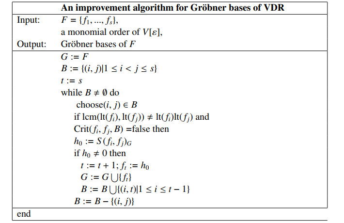
As a special ring with zero divisors, the dual noetherian valuation domain has attracted much attention from scholars. This article aims at to improve the Buchberger's algorithm over the dual noetherian valuation domain. We present some criterions that can be applied in the algorithm for computing Gröbner bases, and the criterions may drastically reduce the number of S-polynomials in the course of the algorithm. In addition, we clearly demonstrate the improvement with an example.

References

[1]	B. Buchberger, An Algorithmic Method in Polynomial Ideal Theory, Reidel Publishing Company, Dodrecht Boston Lancaster, 1985.
[2]	B. Buchberger, A criterion for detecting unnecessary reductions in the construction of Gröbner bases, in Symbolic and Algebraic Computation: EUROSM'79, An International Symposium on Symbolic and Algebraic Manipulation, Springer, Berlin Heidelberg, (1979), 3–21.
[3]	L. Zheng, D. Li, J. Liu, An improvement for GVW, J. Syst. Sci. Complexity, 35 (2022), 427–436. https://doi.org/10.1007/s11424-021-9051-5 doi: 10.1007/s11424-021-9051-5
[4]	L. Zheng, J. Liu, W. Liu, D. Li, A new signature-based algorithms for computing Gröbner bases, J. Syst. Sci. Complexity, 28 (2015), 210–221. https://doi.org/10.1007/s11424-015-2260-z doi: 10.1007/s11424-015-2260-z
[5]	D. Li, J. Liu, L. Zheng, A zero-dimensional valuation ring is 1- Gröbner, J. Algebra, 484 (2017), 334–343. https://doi.org/10.1016/j.jalgebra.2017.04.015 doi: 10.1016/j.jalgebra.2017.04.015
[6]	S. Monceur, I. Yengui, On the leading terms ideal of polynomial ideal over a valuation ring, J. Algebra, 351 (2012), 382–389. https://doi.org/10.1016/j.jalgebra.2011.11.015 doi: 10.1016/j.jalgebra.2011.11.015
[7]	F. Xiao, D. Lu, D. Wang, Solving multivariate polynomial matrix Diophantine equations with Gröbner basis method, J. Syst. Sci. Complexity, 35 (2022), 413–426. https://doi.org/10.1007/s11424-021-0072-x doi: 10.1007/s11424-021-0072-x
[8]	K. Deepak, Y. Cai, An algorithm for computing a Gröbner basis of a polynomial ideal over a ring with zero divisors, Math. Comput. Sci., 2 (2009), 601–634. https://doi.org/10.1007/s11786-009-0072-z doi: 10.1007/s11786-009-0072-z
[9]	E. Golod, On noncommutative Groöbner bases over rings, Math. Sci., 173 (1999), 29–60. https://doi/10.1007/s10958-007-0420-y doi: 10.1007/s10958-007-0420-y
[10]	I. Yengui, Dynamical Gröbner bases, J. Algebra, 301 (2006), 447–458. https://doi/10.1016/j.jalgebra.2006.01.051 doi: 10.1016/j.jalgebra.2006.01.051
[11]	I. Yengui, Corrigendum to "Dynamical Gröbner bases" [J. Algebra 301 (2) (2006) 447–458] and to "Dynamical Gröbner bases over Dedekind rings" [J. Algebra 324 (1) (2010) 12–24], J. Algebra, 339 (2011), 370–375. https://doi/10.1016/j.jalgebra.2011.05.004 doi: 10.1016/j.jalgebra.2011.05.004
[12]	D. M. Li, J. W. Liu, A Gröbner basis algorithm for ideals over zero-dimensional valuation rings, J. Syst. Sci. Complexity, 34 (2021), 2470–2483. https://doi/10.1007/s11424-020-0010-3 doi: 10.1007/s11424-020-0010-3
[13]	O. Wienand, Algorithms for symbolic computation and their applications-standard bases over rings and rank tests in statistics, 2011.
[14]	A. Bouesso, Gröbner bases over a dual valuation domain, Int. J. Algebra, 7 (2013), 539–548.
[15]	T. Markwig, Y. Ren, O. Wienand, Standard bases in mixed power series and polynomial rings over rings, J. Symb. Comput., 79 (2017), 119–139. https://doi/10.1016/j.jsc.2016.08.009 doi: 10.1016/j.jsc.2016.08.009

Reader Comments

Your name:*

Email:*
© 2023 the Author(s), licensee AIMS Press. This is an open access article distributed under the terms of the Creative Commons Attribution License (http://creativecommons.org/licenses/by/4.0)