The exact solutions of the fractional-stochastic Fokas-Lenells equation in optical fiber communication

Sahar Albosaily; Wael Mohammed; Mahmoud El-Morshedy; Sahar Albosaily; Wael Mohammed; Mahmoud El-Morshedy

doi:10.3934/era.2023180

Electronic Research Archive

2023, Volume 31, Issue 6: 3552-3567. doi: 10.3934/era.2023180

Previous Article Next Article

Research article Special Issues

The exact solutions of the fractional-stochastic Fokas-Lenells equation in optical fiber communication

1.
Department of Mathematics, Collage of Science, University of Ha'il, Ha'il 2440, Saudi Arabia
2.
Department of Mathematics, Faculty of Science, Mansoura University, Mansoura 35516, Egypt
3.
Department of Mathematics, College of Science and Humanities in Al-Kharj, Prince Sattam bin Abdulaziz University, Al-Kharj 11942, Saudi Arabia
4.
Department of Statistics and Computer Science, Faculty of Science, Mansoura University, Mansoura 35516, Egypt

Received: 21 January 2023 Revised: 27 March 2023 Accepted: 29 March 2023 Published: 23 April 2023

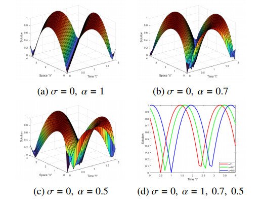
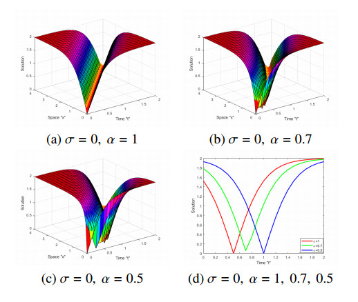
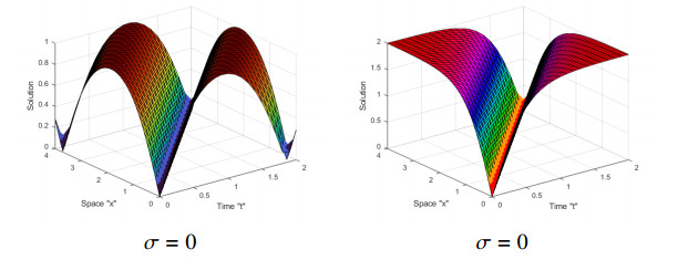
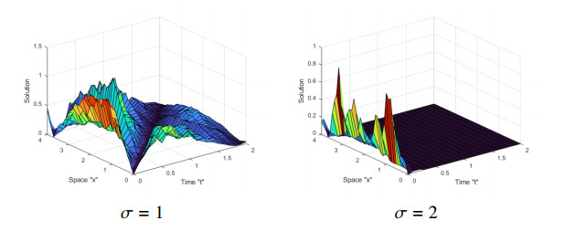
The fractional-stochastic Fokas-Lenells equation (FSFLE) in the Stratonovich sense is taken into account here. The modified mapping method is used to generate new trigonometric, hyperbolic, elliptic and rational stochastic fractional solutions. Because the Fokas-Lenells equation has many implementations in telecommunication modes, complex system theory, quantum field theory, and quantum mechanics, the obtained solutions can be employed to describe a wide range of exciting physical phenomena. We plot several 2D and 3D diagrams to demonstrate how multiplicative noise and fractional derivatives affect the analytical solutions of the FSFLE. Also, we show how multiplicative noise at zero stabilizes FSFLE solutions.

Keywords:

Citation: Sahar Albosaily, Wael Mohammed, Mahmoud El-Morshedy. The exact solutions of the fractional-stochastic Fokas-Lenells equation in optical fiber communication[J]. Electronic Research Archive, 2023, 31(6): 3552-3567. doi: 10.3934/era.2023180

Related Papers:

[1]	Shasha Bian, Yitong Pei, Boling Guo . Numerical simulation of a generalized nonlinear derivative Schrödinger equation. Electronic Research Archive, 2022, 30(8): 3130-3152. doi: 10.3934/era.2022159
[2]	Stephen A. Whitmore, Cara I. Borealis, Max W. Francom . Minimally-intrusive, dual-band, fiber-optic sensing system for high-enthalpy exhaust plumes. Electronic Research Archive, 2024, 32(4): 2541-2597. doi: 10.3934/era.2024117
[3]	Ping Zhou, Hossein Jafari, Roghayeh M. Ganji, Sonali M. Narsale . Numerical study for a class of time fractional diffusion equations using operational matrices based on Hosoya polynomial. Electronic Research Archive, 2023, 31(8): 4530-4548. doi: 10.3934/era.2023231
[4]	Yuchen Zhu . Blow-up of solutions for a time fractional biharmonic equation with exponentional nonlinear memory. Electronic Research Archive, 2024, 32(11): 5988-6007. doi: 10.3934/era.2024278
[5]	Seda IGRET ARAZ, Mehmet Akif CETIN, Abdon ATANGANA . Existence, uniqueness and numerical solution of stochastic fractional differential equations with integer and non-integer orders. Electronic Research Archive, 2024, 32(2): 733-761. doi: 10.3934/era.2024035
[6]	Yaning Li, Mengjun Wang . Well-posedness and blow-up results for a time-space fractional diffusion-wave equation. Electronic Research Archive, 2024, 32(5): 3522-3542. doi: 10.3934/era.2024162
[7]	Hao Wen, Yantao Luo, Jianhua Huang, Yuhong Li . Stochastic travelling wave solution of the $ N $-species cooperative systems with multiplicative noise. Electronic Research Archive, 2023, 31(8): 4406-4426. doi: 10.3934/era.2023225
[8]	Janarthanan Ramadoss, Asma Alharbi, Karthikeyan Rajagopal, Salah Boulaaras . A fractional-order discrete memristor neuron model: Nodal and network dynamics. Electronic Research Archive, 2022, 30(11): 3977-3992. doi: 10.3934/era.2022202
[9]	Shufen Zhao, Xiaoqian Li, Jianzhong Zhang . S-asymptotically $ \omega $-periodic solutions in distribution for a class of stochastic fractional functional differential equations. Electronic Research Archive, 2023, 31(2): 599-614. doi: 10.3934/era.2023029
[10]	E. A. Abdel-Rehim . The time evolution of the large exponential and power population growth and their relation to the discrete linear birth-death process. Electronic Research Archive, 2022, 30(7): 2487-2509. doi: 10.3934/era.2022127

Abstract

1. Introduction

Nonlinear evolution equations (NEEs) are used extensively in engineering and scientific fields, including wave propagation phenomena, quantum mechanics, shallow water wave propagation, chemical kinematics, solid-state physics, optical fibers, fluid mechanics, plasma physics, heat flow and so on. Recently, much research on NEEs has focused on existence, uniqueness, convergence and finding solutions: for example, ^{[1,2,3,4,5,6,7,8,9,10,11]}, and the references therein. One of the essential physical issues for NEEs is obtaining traveling wave solutions. Therefore, the looking for mathematical techniques to generate exact solutions to NEEs has become a significant and necessary task in nonlinear sciences. Recently, various techniques for dealing with NEEs have been established, such as the exp-function method ^[12], perturbation method ^[13,14], sine-cosine method ^[15,16], spectral methods ^[17], tanh-sech method ^[18,19], Jacobi elliptic function ^[20], Hirota's method ^[21], $exp(-\phi (\varsigma))$ -expansion method ^[22], extended trial equation method ^[23,24], $(G^{\prime }/G)$ -expansion method ^[25,26], etc.

In recent years, the use of fractional differential equations has grown due to their wide range of applications in fields such as control theory, fluid flow, finance, electrical networks, solid state physics, chemical kinematics, optical fiber, plasma physics, signal processing, and biological populations. A number of mathematicians have proposed various types of fractional derivatives. These types include, the new truncated M-fractional derivative, Caputo fractional derivative, Riemann-Liouville fractional derivative, Grunwald-Letnikov fractional derivative, He's fractional derivative, Riesz fractional derivatives, the Weyl derivative and conformable fractional definitions ^{[27,28,29,30,31,32,33,34]}.

Khalil et al. ^[32] have developed a new derivative operator known as the conformable derivative (CD). From this point, let us define the CD for the function $u:[0, \infty)\rightarrow \mathbb{R}$ of order $\beta \in (0, 1]$ as follows:

$\begin{equation*} \mathcal{D}_{z}^{\beta }u(z) = \lim\limits_{h\rightarrow 0}\frac{u(z+hz^{1-\beta })-u(z)}{h}. \end{equation*}$

The CD satisfies the following properties for any constants $a$ and $b$ :

1) $\mathcal{D}_{z}^{\beta }[au(z)+bv(z)] = a\mathcal{D}_{z}^{\beta }u(z)+b \mathcal{D}_{z}^{\beta }v(z)\$ , 2) $\mathcal{D}_{z}^{\beta }[a] = 0,$

3) $\mathcal{D}_{z}^{\beta }[z^{a}] = az^{a-\beta }, \$ 4) $\ \mathcal{D} _{z}^{\beta }u(z) = z^{1-\beta }\frac{du}{dz}.$

In contrast, stochastic partial differential equations (SPDEs) are models for spatiotemporal physical, biological and chemical systems that are sensitive to random influences. In the past few decades, these models have been the subject of extensive research. It has been emphasized how crucial it is to take stochastic effects into account when modeling complex systems. For instance, there is rising interest in employing SPDEs to represent complex phenomena mathematically in the fields of finance, mechanical and electrical engineering, biophysics, information systems, materials sciences, condensed matter physics, and climate systems ^[35,36].

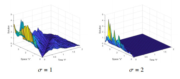
Therefore, it is crucial to consider NEEs with fractional derivatives and for some stochastic force. Here, we consider the fractional-stochastic Fokas-Lenells equation (FSFLE):

$\begin{equation} \mathcal{D}_{x}^{\alpha }\Phi _{t}-\gamma _{1}\mathcal{D}_{xx}^{\alpha }\Phi -2i\gamma _{2}\mathcal{D}_{x}^{\alpha }\Phi +\vartheta \left\vert \Phi \right\vert ^{2}(\Phi +i\rho \mathcal{D}_{x}^{\alpha }\Phi )+\sigma \mathcal{ D}_{x}^{\alpha }\Phi \circ W_{t} = 0, \end{equation}$

(1.1)

where $\Phi (x, t)$ gives the complex field, $\gamma _{1}, \ \gamma _{2}$ and $\rho$ are positive constants, $\vartheta = \pm 1, \ W$ is the standard Wiener process, $\ \sigma$ is the strength of the noise, and $\Phi \circ dW$ is multiplicative noise in the Stratonovich sense.

If we put $\sigma = 0$ and $\alpha = 1$ , then we get the Fokas-Lenells equation ^[37,38,39]:

$\begin{equation} \Phi _{xt}-\gamma _{1}\Phi _{xx}-2i\gamma _{2}\Phi _{x}+\vartheta \left\vert \Phi \right\vert ^{2}(\Phi +i\rho \Phi _{x}) = 0. \end{equation}$

(1.2)

Equation (1.2) is one of the most significant equations, and it has many applications in telecommunication models, complex system theory, quantum field theory and quantum mechanics. Also, it appears as a pattern that identifies nonlinear pulse propagation in optical fibers. Demiray and Bulut ^[37] obtained the exact solutions of Eq (1.2) by utilizing the extended trial equation and generalized Kudryashov methods. Meanwhile, Xu and Fan ^[38] used the Riemann-Hilbert problem to obtain the long-time asymptotic behavior of the solution of Eq (1.2).

It is important to note that Stratonovich and Itô ^[40] are the two versions of stochastic integrals that are most frequently used. Modeling problems essentially establish which form is acceptable; nevertheless, once that form is chosen, an equivalent equation of the alternate form can be created utilizing the same solutions. The following correlation can therefore be used to switch between Stratonovich (denoted as $\int_{0}^{t}\Phi \circ dW$ ) and Itô (denoted as $\int_{0}^{t}\Phi dW$ ):

$\begin{equation} \int_{0}^{t}\sigma \Phi (\tau )\circ dW(\tau ) = \int_{0}^{t}\sigma \Phi (\tau )dW(\tau )+\frac{\sigma ^{2}}{2}\int_{0}^{t}\Phi (\tau )d\tau . \end{equation}$

(1.3)

Our aim in this study is to derive the analytical fractional-stochastic solutions of the FSFLE (1.1). The modified mapping method is what we employ to obtain these solutions. Physics researchers would find the solutions very helpful in defining several major physical processes because of the stochastic term and fractional derivatives present in Eq (1.1). Additionally, by using MATLAB software, we introduce numerous graphs to investigate the effects of noise and the fractional derivative on the exact solution of the FSFLE (1.1).

The outline of this paper is as follows: In Section 2, we get the wave equation for the FSFLE (1.1). In Section 3, the modified mapping method is used to get the exact solutions of the FSFLE (1.1). In Section 4, we can see how white noise and the fractional derivative affect the acquired FSFLE solutions. At last, the conclusions of the paper are given.

2. Traveling wave equation for FSFLE

The wave equation for FSFLE (1.1) is obtained by using the wave transformation

$\begin{equation} \Phi (x, t) = \Psi (\eta )e^{i\Theta (\mu )-\sigma W(t)-\sigma ^{2}t}, { \ } \Theta (\mu ) = \frac{\mu _{1}}{\alpha }x^{\alpha }+\mu _{2}t\ \ \text{and} \ \eta = \frac{\eta _{1}}{\alpha }x^{\alpha }+\eta _{2}t, \end{equation}$

(2.1)

where the function $\ \Psi$ is deterministic, and $\mu _{1}, \ \mu _{2}, \ \eta _{1}\$ and $\eta _{2}$ are non-zero constants. We note that

$\begin{eqnarray} \Phi _{t} & = &[\eta _{2}\Psi ^{\prime }+i\mu _{2}\Psi -\sigma \Psi W_{t}+ \frac{1}{2}\sigma ^{2}\Psi -\sigma ^{2}\Psi ]e^{i\Theta (\mu )-\sigma W(t)-\sigma ^{2}t}, \\ & = &[\eta _{2}\Psi ^{\prime }+i\mu _{2}\Psi -\sigma \Psi W_{t}-\frac{1}{2} \sigma ^{2}\Psi ]e^{i\Theta (\mu )-\sigma W(t)-\sigma ^{2}t}, \\ & = &[\eta _{2}\Psi ^{\prime }+i\mu _{2}\Psi -\sigma \Psi \circ W_{t}]e^{i\Theta (\mu )-\sigma W(t)-\sigma ^{2}t}, \end{eqnarray}$

(2.2)

where we used Eq (1.3), and the term $\frac{1}{2}\sigma ^{2}\Psi$ is the Itô correction.

$\begin{equation} \mathcal{D}_{x}^{\alpha }\Phi _{t} = [\eta _{1}\eta _{2}\Psi ^{\prime \prime }+i(\eta _{1}\mu _{2}+\mu _{1}\eta _{2})\Psi ^{\prime }-\sigma (\eta _{1}\Psi ^{\prime }+i\mu _{1}\Psi )\circ W_{t}-\mu _{1}\mu _{2}\Psi ]e^{i\Theta (\mu )-\sigma W(t)-\sigma ^{2}t}, \end{equation}$

(2.3)

and

$\begin{eqnarray} \mathcal{D}_{x}^{\alpha }\Phi & = &(\eta _{1}\Psi ^{\prime }+i\mu _{1}\Psi )e^{i\Theta (\mu )+\sigma W(t)-\sigma ^{2}t}\text{, } \\ \mathcal{D}_{xx}^{\alpha }\Phi & = &(\eta _{1}^{2}\Psi ^{\prime \prime }+2i\mu _{1}\eta _{1}\Psi ^{\prime }-\mu _{1}^{2}\Psi )e^{i\Theta (\mu )-\sigma W(t)-\sigma ^{2}t}. \end{eqnarray}$

(2.4)

Inserting Eqs (2.3) and (2.4) into Eq (1.1), we have the following system:

$\begin{equation} (\eta _{1}\eta _{2}-\gamma _{1}\eta _{1}^{2})\Psi ^{\prime \prime }+(\nu -\mu _{1}\mu _{2}+\gamma _{1}^{2}\mu _{1}+2\gamma _{2}\mu _{1})\Psi -\nu \rho \mu _{1}\Psi ^{3}e^{[-2\sigma W(t)-2\sigma ^{2}t]} = 0, \end{equation}$

(2.5)

and

$\begin{equation} i[(\eta _{1}\mu _{2}+\mu _{1}\eta _{2}-2\gamma _{1}\mu _{1}\eta _{1}-2\gamma _{2}\eta _{1})\Psi ^{\prime }+\nu \rho \eta _{1}\Psi ^{2}\Psi ^{\prime }e^{[-2\sigma W(t)-2\sigma ^{2}t]}] = 0. \end{equation}$

(2.6)

We have, by taking the expectation on both sides,

$\begin{equation} (\eta _{1}\eta _{2}-\gamma _{1}\eta _{1}^{2})\Psi ^{\prime \prime }+(\nu -\mu _{1}\mu _{2}+\gamma _{1}^{2}\mu _{1}+2\gamma _{2}\mu _{1})\Psi -\nu \rho \mu _{1}\Psi ^{3}e^{-2\sigma ^{2}t}\mathbb{E}e^{-2\sigma W(t)} = 0, \end{equation}$

(2.7)

and

$\begin{equation} i[(\eta _{1}\mu _{2}+\mu _{1}\eta _{2}-2\gamma _{1}\mu _{1}\eta _{1}-2\gamma _{2}\eta _{1})\Psi ^{\prime }+\nu \rho \eta _{1}\Psi ^{2}\Psi ^{\prime }e^{-2\sigma ^{2}t}\mathbb{E}e^{-2\sigma W(t)}] = 0. \end{equation}$

(2.8)

Since $W(t)$ is normal distribution, then $\mathbb{E(}e^{2kW(t)}) = e^{2k^{2}t}$ for any real number $k$ . Therefore, Eqs (2.7) and (2.8) become

(2.9)

$\begin{equation} i[(\eta _{1}\mu _{2}+\mu _{1}\eta _{2}-2\gamma _{1}\mu _{1}\eta _{1}-2\gamma _{2}\eta _{1})\Psi ^{\prime }+\nu \rho \eta _{1}\Psi ^{2}\Psi ^{\prime }] = 0. \end{equation}$

(2.10)

From the imaginary part of Eq (2.10), we obtained

$\begin{equation*} \eta _{2} = \frac{1}{\mu _{1}}(-\eta _{1}\mu _{2}+2\gamma _{1}\mu _{1}\eta _{1}+2\gamma _{2}\eta _{1}-\nu \rho \eta _{1}\Psi ^{2}). \end{equation*}$

while the real part is given by

$\begin{equation} \Psi ^{\prime \prime }+A\Psi -B\Psi ^{3} = 0, \end{equation}$

(2.11)

where

$\begin{equation*} A = \frac{(\nu -\mu _{1}\mu _{2}+\gamma _{1}^{2}\mu _{1}+2\gamma _{2}\mu _{1}) }{(\eta _{1}\eta _{2}-\gamma _{1}\eta _{1}^{2})}\text{, and }B = \frac{\nu \rho \mu _{1}}{(\eta _{1}\eta _{2}-\gamma _{1}\eta _{1}^{2})}. \end{equation*}$

3. Exact solutions of FSFLE

In this section, we apply the modified mapping method stated in ^[41]. Assuming that the solutions of Eq (2.11) have the form

$\begin{equation} \Psi (\eta ) = \sum\limits_{i = 0}^{N}\ell _{i}\varphi ^{i}(\eta )+\sum\limits_{i = 1}^{N}\hslash _{i}\varphi ^{-i}(\eta ), \end{equation}$

(3.1)

where $\ell _{i}$ and $\hslash _{i}$ are unknown constants to be evaluated for $i = 1, 2, ..\ell _{N},$ and $\varphi$ satisfies the first type of the elliptic equation

$\begin{equation} \varphi ^{\prime } = \sqrt{r+q\varphi ^{2}+p\varphi ^{4}}, \end{equation}$

(3.2)

where $r, q$ and $\ p$ are real parameters.

First, let us balance $\Psi ^{\prime \prime }$ with $\Psi ^{3}$ in Eq (2.11) to find the parameter $N$ as

$\begin{equation*} N+2 = 3N\Longrightarrow N = 1. \end{equation*}$

With $N = 1$ , Eq (3.2) takes the form

$\begin{equation} \Psi (\eta ) = \ell _{0}+\ell _{1}\varphi (\eta )+\frac{\hslash _{1}}{\varphi (\eta )}. \end{equation}$

(3.3)

Differentiating Eq (3.3) twice and using (3.2), we get

$\begin{equation} \Psi ^{\prime \prime } = \ell _{1}(q\varphi +2p\varphi ^{3})+\hslash _{1}(q\varphi ^{-1}+2r\varphi ^{-3}). \end{equation}$

(3.4)

Putting Eqs (3.3) and (3.4) into Eq (2.11) we have

$\begin{eqnarray*} &&(2\ell _{1}p-B\ell _{1}^{3})\varphi ^{3}-3B\ell _{0}\ell _{1}^{2}\varphi ^{2}+(\ell _{1}q-3B\ell _{0}^{2}\ell _{1}-3B\hslash _{1}\ell _{1}^{2}+\ell _{1}A)\varphi \\ &&+(A\ell _{0}-B\ell _{0}^{3}-6B\ell _{0}\ell _{1}\hslash _{1})+(A\hslash _{1}+\hslash _{1}q-3B\ell _{0}^{2}\hslash _{1}-3B\ell _{1}\hslash _{1}^{2})\varphi ^{-1} \\ &&-3B\hslash _{1}^{2}\varphi ^{-2}+(2r\hslash _{1}-B\hslash _{1}^{3})\varphi ^{-3} = 0. \end{eqnarray*}$

Comparing each coefficient of $\varphi ^{k}$ and $\varphi ^{-k}$ with zero for $k = 3, 2, 1, 0,$ we attain

$\begin{equation*} 2\ell _{1}p-B\ell _{1}^{3} = 0, \end{equation*}$

$\begin{equation*} -3B\ell _{0}\ell _{1}^{2} = 0, \end{equation*}$

$\begin{equation*} \ell _{1}q-3B\ell _{0}^{2}\ell _{1}-3B\hslash _{1}\ell _{1}^{2}+\ell _{1}A = 0, \end{equation*}$

$\begin{equation*} A\ell _{0}-B\ell _{0}^{3}-6B\ell _{0}\ell _{1}\hslash _{1} = 0, \end{equation*}$

$\begin{equation*} A\hslash _{1}+\hslash _{1}q-3B\ell _{0}^{2}\hslash _{1}-3B\ell _{1}\hslash _{1}^{2} = 0, \end{equation*}$

$\begin{equation*} -3B\ell _{0}\hslash _{1}^{2} = 0 \end{equation*}$

and

$\begin{equation*} 2r\hslash _{1}-B\hslash _{1}^{3} = 0. \end{equation*}$

When we solve these equations, we get three different families:

First family:

$\begin{equation} \ell _{0} = 0, \ \ \ell _{1} = \pm \sqrt{\frac{2p}{B}}, \ \hslash _{1} = 0, \ \ q = -A. \end{equation}$

(3.5)

Second family:

$\begin{equation} \ell _{0} = 0, \ \ \ell _{1} = 0, \ \hslash _{1} = \pm \sqrt{\frac{2r}{B}}, \ \ q = -A. \end{equation}$

(3.6)

Third family:

$\begin{equation} \ell _{0} = 0, \ \ \ell _{1} = \pm \sqrt{\frac{2p}{B}}, \ \hslash _{1} = \pm \sqrt{ \frac{2r}{B}}, \ \ q = 6\sqrt{pr}-A. \end{equation}$

(3.7)

First family: The solution of Eq (2.11), by utilizing Eqs (3.3) and (3.5), takes the form

$\begin{equation} \Phi (x, t) = \pm \sqrt{\frac{2p}{B}}\varphi (\eta )e^{i\Theta (\mu )-\sigma W(t)-\sigma ^{2}t}. \end{equation}$

(3.8)

There are many cases depending on $p > 0:$

Case 1-1: If $p = \kappa ^{2}, \ q = -(1+\kappa ^{2})$ and $\ r = 1,$ then $\varphi (\eta) = sn(\eta).$ In this case the solution of FSFLE (1.1), by utilizing Eq (3.8), is

$\begin{equation} \Phi (x, t) = \pm \kappa \sqrt{\frac{2}{B}}sn(\frac{\eta _{1}}{\alpha } x^{\alpha }+\eta _{2}t)e^{i\Theta (\mu )-\sigma W(t)-\sigma ^{2}t}. \end{equation}$

(3.9)

If $\kappa \rightarrow 1,$ then Eq (3.9) transfers to

$\begin{equation} \Phi (x, t) = \pm \sqrt{\frac{2}{B}}\tanh (\frac{\eta _{1}}{\alpha }x^{\alpha }+\eta _{2}t)e^{i\Theta (\mu )-\sigma W(t)-\sigma ^{2}t}. \end{equation}$

(3.10)

Case 1-2: If $p = 1, \ q = 2\kappa ^{2}-1$ and $\ r = -\kappa ^{2}(1-\kappa ^{2}),$ then $\varphi (\eta) = ds(\eta).$ In this case the solution of FSFLE (1.1), by using Eq (3.8), is

$\begin{equation} \Phi (x, t) = \pm \sqrt{\frac{2}{B}}ds(\frac{\eta _{1}}{\alpha }x^{\alpha }+\eta _{2}t)e^{i\Theta (\mu )-\sigma W(t)-\sigma ^{2}t}. \end{equation}$

(3.11)

If $\kappa \rightarrow 1,$ then Eq (3.11) transfers to

$\begin{equation} \Phi (x, t) = \pm \sqrt{\frac{2}{B}}\text{csch}(\frac{\eta _{1}}{\alpha } x^{\alpha }+\eta _{2}t)e^{i\Theta (\mu )-\sigma W(t)-\sigma ^{2}t}. \end{equation}$

(3.12)

If $\kappa \rightarrow 0,$ then Eq (3.11) transfers to

$\begin{equation} \Phi (x, t) = \pm \sqrt{\frac{2}{B}}\csc (\frac{\eta _{1}}{\alpha }x^{\alpha }+\eta _{2}t)e^{i\Theta (\mu )-\sigma W(t)-\sigma ^{2}t}. \end{equation}$

(3.13)

Case 1-3: If $p = 1, \ q = 2-\kappa ^{2}$ and $\ r = (1-\kappa ^{2}),$ then $\varphi (\eta) = cs(\eta).$ In this case the solution of FSFLE (1.1), by utilizing Eq (3.8), is

$\begin{equation} \Phi (x, t) = \pm \sqrt{\frac{2}{B}}cs(\frac{\eta _{1}}{\alpha }x^{\alpha }+\eta _{2}t)e^{i\Theta (\mu )-\sigma W(t)-\sigma ^{2}t}. \end{equation}$

(3.14)

If $\kappa \rightarrow 1,$ then Eq (3.14) transfers to

$\begin{equation} \Phi (x, t) = \pm \sqrt{\frac{2}{B}}\text{csch}(\frac{\eta _{1}}{\alpha } x^{\alpha }+\eta _{2}t)e^{i\Theta (\mu )-\sigma W(t)-\sigma ^{2}t}. \end{equation}$

(3.15)

When $\kappa \rightarrow 0,$ then Eq (3.14) transfers to

$\begin{equation} \Phi (x, t) = \pm \sqrt{\frac{2}{B}}\cot (\frac{\eta _{1}}{\alpha }x^{\alpha }+\eta _{2}t)e^{i\Theta (\mu )-\sigma W(t)-\sigma ^{2}t}. \end{equation}$

(3.16)

Case 1-4: If $p = \frac{\kappa ^{2}}{4}, \ q = \frac{(\kappa ^{2}-2)}{2}$ and $\ r = \frac{1}{4},$ then $\varphi (\eta) = \frac{sn(\eta)}{1+dn(\eta)}.$ In this case the solution of FSFLE (1.1), by using Eq (3.8), is

$\begin{equation} \Phi (x, t) = \pm \kappa \sqrt{\frac{1}{2B}}\frac{sn(\frac{\eta _{1}}{\alpha } x^{\alpha }+\eta _{2}t)}{1+dn(\frac{\eta _{1}}{\alpha }x^{\alpha }+\eta _{2}t)}e^{i\Theta (\mu )-\sigma W(t)-\sigma ^{2}t}. \end{equation}$

(3.17)

If $\kappa \rightarrow 1,$ then Eq (3.17) transfers to

$\begin{equation} \Phi (x, t) = \pm \sqrt{\frac{1}{2B}}\frac{\tanh (\frac{\eta _{1}}{\alpha } x^{\alpha }+\eta _{2}t)}{1+\text{sech}(\frac{\eta _{1}}{\alpha }x^{\alpha }+\eta _{2}t)}e^{i\Theta (\mu )-\sigma W(t)-\sigma ^{2}t}. \end{equation}$

(3.18)

Case 1-5: If $p = \frac{(1-\kappa ^{2})^{2}}{4}, \ q = \frac{(1-\kappa ^{2})^{2}}{2}$ and $\ r = \frac{1}{4},$ then $\varphi (\eta) = \frac{sn(\eta)}{ dn(\eta)+cn(\eta)}.$ In this case the solution of FSFLE (1.1), by using Eq (3.8), is

$\begin{equation} \Phi (x, t) = \pm (1-\kappa ^{2})\sqrt{\frac{1}{2B}}[\frac{sn(\frac{\eta _{1}}{ \alpha }x^{\alpha }+\eta _{2}t)}{dn(\frac{\eta _{1}}{\alpha }x^{\alpha }+\eta _{2}t)+cn(\frac{\eta _{1}}{\alpha }x^{\alpha }+\eta _{2}t)} ]e^{i\Theta (\mu )-\sigma W(t)-\sigma ^{2}t}. \end{equation}$

(3.19)

If $\kappa \rightarrow 0,$ then Eq (3.19) transfers to

$\begin{equation} \Phi (x, t) = \pm \sqrt{\frac{1}{2B}}[\frac{\sin (\frac{\eta _{1}}{\alpha } x^{\alpha }+\eta _{2}t)}{1+\cos (\frac{\eta _{1}}{\alpha }x^{\alpha }+\eta _{2}t)}]e^{i\Theta (\mu )-\sigma W(t)-\sigma ^{2}t}. \end{equation}$

(3.20)

Case 1-6: If $p = \frac{1-\kappa ^{2}}{4}, \ q = \frac{(1-\kappa ^{2})}{2 }$ and $\ r = \frac{1-\kappa ^{2}}{4},$ then $\varphi (\eta) = \frac{cn(\eta)}{ 1+sn(\eta)}.\$ In this case the solution of FSFLE (1.1), by using Eq (3.8), is

$\begin{equation} \Phi (x, t) = \pm \sqrt{\frac{2}{B}}\frac{cn(\frac{\eta _{1}}{\alpha }x^{\alpha }+\eta _{2}t)}{1+sn(\frac{\eta _{1}}{\alpha }x^{\alpha }+\eta _{2}t)} ]e^{i\Theta (\mu )-\sigma W(t)-\sigma ^{2}t}. \end{equation}$

(3.21)

When $\kappa \rightarrow 0,$ then Eq (3.21) transfers to

$\begin{equation} \Phi (x, t) = \pm \frac{1}{2}\sqrt{\frac{2}{B}}\frac{\cos (\frac{\eta _{1}}{ \alpha }x^{\alpha }+\eta _{2}t)}{1+\sin (\frac{\eta _{1}}{\alpha }x^{\alpha }+\eta _{2}t)}]e^{i\Theta (\mu )-\sigma W(t)-\sigma ^{2}t}. \end{equation}$

(3.22)

Case 1-7: If $p = 1, \ q = 0$ and $\ r = 0,$ then $\varphi (\eta) = \frac{c}{ \eta }.\$ In this case the solution of FSFLE (1.1), by utilizing Eq (3.8), is

$\begin{equation} \Phi (x, t) = \pm \sqrt{\frac{2}{B}}\frac{c}{(\frac{\eta _{1}}{\alpha } x^{\alpha }+\eta _{2}t)}]e^{i\Theta (\mu )-\sigma W(t)-\sigma ^{2}t}. \end{equation}$

(3.23)

Second family: The solution of Eq (2.11), by using Eqs (3.3) and (3.6), takes the form

$\begin{equation} \Phi (x, t) = \pm \sqrt{\frac{2r}{B}}\frac{1}{\varphi (\eta )}e^{i\Theta (\mu )-\sigma W(t)-\sigma ^{2}t}. \end{equation}$

(3.24)

There are many cases depending on $r > 0:$

Case 2-1: If $p = \kappa ^{2}, \ q = -(1+\kappa ^{2})$ and $\ r = 1,$ then $\varphi (\eta) = sn(\eta).$ In this case the solution of FSFLE (1.1), by utilizing Eq (3.24), is

$\begin{equation} \Phi (x, t) = \pm \sqrt{\frac{2}{B}}\frac{1}{sn(\frac{\eta _{1}}{\alpha } x^{\alpha }+\eta _{2}t)}e^{i\Theta (\mu )-\sigma W(t)-\sigma ^{2}t}. \end{equation}$

(3.25)

If $\kappa \rightarrow 1,$ then Eq (3.25) transfers to

$\begin{equation} \Phi (x, t) = \pm \sqrt{\frac{2}{B}}\coth (\frac{\eta _{1}}{\alpha }x^{\alpha }+\eta _{2}t)e^{i\Theta (\mu )-\sigma W(t)-\sigma ^{2}t}. \end{equation}$

(3.26)

Case 2-2: If $p = 1, \ q = 2-\kappa ^{2}$ and $\ r = (1-\kappa ^{2}),$ then $\varphi (\eta) = cs(\eta).$ In this case the solution of FSFLE (1.1), by utilizing Eq (3.24), is

$\begin{equation} \Phi (x, t) = \pm \sqrt{\frac{2(1-\kappa ^{2})}{B}}\frac{1}{cs(\frac{\eta _{1}}{ \alpha }x^{\alpha }+\eta _{2}t)}e^{i\Theta (\mu )-\sigma W(t)-\sigma ^{2}t}. \end{equation}$

(3.27)

When $\kappa \rightarrow 0,$ then Eq (3.27) transfers to

$\begin{equation} \Phi (x, t) = \pm \sqrt{\frac{2}{B}}\tan (\frac{\eta _{1}}{\alpha }x^{\alpha }+\eta _{2}t)e^{i\Theta (\mu )-\sigma W(t)-\sigma ^{2}t}. \end{equation}$

(3.28)

Case 2-3: If $p = -\kappa ^{2}, \ q = 2\kappa ^{2}-1$ and $\ r = (1-\kappa ^{2}),$ then $\varphi (\eta) = cn(\mu).$ In this case the solution of FSFLE (1.1), by utilizing Eq (3.24), is

$\begin{equation} \Phi (x, t) = \pm \sqrt{\frac{2(1-\kappa ^{2})}{B}}\frac{1}{cn(\frac{\eta _{1}}{ \alpha }x^{\alpha }+\eta _{2}t)}e^{i\Theta (\mu )-\sigma W(t)-\sigma ^{2}t}. \end{equation}$

(3.29)

If $\kappa \rightarrow 0,$ then Eq (3.31) transfers to

$\begin{equation} \Phi (x, t) = \pm \sqrt{\frac{2}{B}}\sec (\frac{\eta _{1}}{\alpha }x^{\alpha }+\eta _{2}t)e^{i\Theta (\mu )-\sigma W(t)-\sigma ^{2}t}. \end{equation}$

(3.30)

Case 2-4: If $p = \frac{\kappa ^{2}}{4}, \ q = \frac{(\kappa ^{2}-2)}{2}$ and $\ r = \frac{1}{4},$ then $\varphi (\eta) = \frac{sn(\eta)}{1+dn(\eta)}.$ In this case the solution of FSFLE (1.1), by using Eq (3.24), is

$\begin{equation} \Phi (x, t) = \pm \sqrt{\frac{1}{2B}}\frac{1+dn(\frac{\eta _{1}}{\alpha } x^{\alpha }+\eta _{2}t)}{sn(\frac{\eta _{1}}{\alpha }x^{\alpha }+\eta _{2}t)} e^{i\Theta (\mu )-\sigma W(t)-\sigma ^{2}t}. \end{equation}$

(3.31)

If $\kappa \rightarrow 1,$ then Eq (3.31) transfers to

$\begin{equation} \Phi (x, t) = \pm \sqrt{\frac{1}{2B}}[\coth (\frac{\eta _{1}}{\alpha }x^{\alpha }+\eta _{2}t)+\text{csch}(\frac{\eta _{1}}{\alpha }x^{\alpha }+\eta _{2}t)]e^{i\Theta (\mu )-\sigma W(t)-\sigma ^{2}t}. \end{equation}$

(3.32)

Case 2-5: If $p = \frac{1-\kappa ^{2}}{4}, \ q = \frac{(1-\kappa ^{2})}{2 }$ and $\ r = \frac{1-\kappa ^{2}}{4},$ then $\varphi (\eta) = \frac{cn(\eta)}{ 1+sn(\eta)}.\$ In this case the solution of FSFLE (1.1), by utilizing Eq (3.8), is

$\begin{equation} \Phi (x, t) = \pm \sqrt{\frac{1-\kappa ^{2}}{2B}}\frac{1+sn(\frac{\eta _{1}}{ \alpha }x^{\alpha }+\eta _{2}t)}{cn(\frac{\eta _{1}}{\alpha }x^{\alpha }+\eta _{2}t)}]e^{i\Theta (\mu )-\sigma W(t)-\sigma ^{2}t}. \end{equation}$

(3.33)

When $\kappa \rightarrow 0,$ then Eq (3.33) transfers to

$\begin{equation} \Phi (x, t) = \pm \sqrt{\frac{2}{B}}[\sec (\frac{\eta _{1}}{\alpha }x^{\alpha }+\eta _{2}t)\pm \tan cn(\frac{\eta _{1}}{\alpha }x^{\alpha }+\eta _{2}t)]e^{i\Theta (\mu )-\sigma W(t)-\sigma ^{2}t}. \end{equation}$

(3.34)

Case 2-6: If $p = \frac{(1-\kappa ^{2})^{2}}{4}, \ q = \frac{(1-\kappa ^{2})^{2}}{2}$ and $\ r = \frac{1}{4},$ then $\varphi (\eta) = \frac{sn(\eta)}{ dn(\eta)+cn(\eta)}.$ In this case the solution of FSFLE (1.1), by using Eq (3.24), is

$\begin{equation} \Phi (x, t) = \pm \sqrt{\frac{1}{2B}}[\frac{dn(\frac{\eta _{1}}{\alpha } x^{\alpha }+\eta _{2}t)+cn(\frac{\eta _{1}}{\alpha }x^{\alpha }+\eta _{2}t)}{ sn(\frac{\eta _{1}}{\alpha }x^{\alpha }+\eta _{2}t)}]e^{i\Theta (\mu )-\sigma W(t)-\sigma ^{2}t}. \end{equation}$

(3.35)

If $\kappa \rightarrow 0,$ then Eq (3.35) transfers to

$\begin{equation} \Phi (x, t) = \pm \sqrt{\frac{1}{2B}}[\csc (\frac{\eta _{1}}{\alpha }x^{\alpha }+\eta _{2}t)+\cot (\frac{\eta _{1}}{\alpha }x^{\alpha }+\eta _{2}t)]e^{i\Theta (\mu )-\sigma W(t)-\sigma ^{2}t}. \end{equation}$

(3.36)

If $\kappa \rightarrow 1,$ then Eq (3.35) transfers to

$\begin{equation} \Phi (x, t) = \pm \sqrt{\frac{2}{B}}\text{csch}(\frac{\eta _{1}}{\alpha } x^{\alpha }+\eta _{2}t)e^{i\Theta (\mu )-\sigma W(t)-\sigma ^{2}t}. \end{equation}$

(3.37)

Third family: The solution of Eq (2.11), using Eqs (3.3) and (3.7), takes the form

$\begin{equation} \Phi (x, t) = [\pm \sqrt{\frac{2p}{B}}\varphi (\eta )\pm \sqrt{\frac{2r}{B}} \frac{1}{\varphi (\eta )}]e^{i\Theta (\mu )-\sigma W(t)-\sigma ^{2}t}. \end{equation}$

(3.38)

There are many cases depending on $r > 0:$

Case 3-1: If $p = \kappa ^{2}, \ q = -(1+\kappa ^{2})$ and $\ r = 1,$ then $\varphi (\eta) = sn(\eta).$ In this case the solution of FSFLE (1.1), by utilizing Eq (3.38), is

$\begin{equation} \Phi (x, t) = \pm \sqrt{\frac{2}{B}}[\kappa sn(\frac{\eta _{1}}{\alpha } x^{\alpha }+\eta _{2}t)+\frac{1}{sn(\frac{\eta _{1}}{\alpha }x^{\alpha }+\eta _{2}t)}]e^{i\Theta (\mu )-\sigma W(t)-\sigma ^{2}t}. \end{equation}$

(3.39)

If $\kappa \rightarrow 1,$ then Eq (3.39) transfers to

$\begin{equation} \Phi (x, t) = \pm \lbrack \sqrt{\frac{2}{B}}\tanh (\frac{\eta _{1}}{\alpha } x^{\alpha }+\eta _{2}t)+\sqrt{\frac{2}{B}}\coth (\frac{\eta _{1}}{\alpha } x^{\alpha }+\eta _{2}t)]e^{i\Theta (\mu )-\sigma W(t)-\sigma ^{2}t}. \end{equation}$

(3.40)

Case 3-2: If $p = 1, \ q = 2-\kappa ^{2}$ and $\ r = (1-\kappa ^{2}),$ then $\varphi (\eta) = cs(\eta).$ In this case the solution of FSFLE (1.1), by using Eq (3.38), is

$\begin{equation} \Phi (x, t) = \pm \lbrack \sqrt{\frac{2}{B}}cs(\eta )+\sqrt{\frac{2(1-\kappa ^{2})}{B}}\frac{1}{cs(\eta )}e^{i\Theta (\mu )-\sigma W(t)-\sigma ^{2}t}, \end{equation}$

(3.41)

where $\eta = \frac{\eta _{1}}{\alpha }x^{\alpha }+\eta _{2}t.\$ When $\kappa \rightarrow 0,$ then Eq (3.41) transfers to

$\begin{equation} \Phi (x, t) = \pm \sqrt{\frac{2}{B}}[\cot (\frac{\eta _{1}}{\alpha }x^{\alpha }+\eta _{2}t)+\tan (\frac{\eta _{1}}{\alpha }x^{\alpha }+\eta _{2}t)]e^{i\Theta (\mu )-\sigma W(t)-\sigma ^{2}t}. \end{equation}$

(3.42)

Case 3-3: If $p = \frac{\kappa ^{2}}{4}, \ q = \frac{(\kappa ^{2}-2)}{2}$ and $\ r = \frac{1}{4},$ then $\varphi (\eta) = \frac{sn(\eta)}{1\pm dn(\eta)}.$ In this case the solution of FSFLE (1.1), by utilizing Eq (3.38), is

$\begin{equation} \Phi (x, t) = \pm \sqrt{\frac{1}{2B}}[\kappa \frac{sn(\eta }{1+dn(\eta )}+\frac{ 1+dn(\eta )}{sn(\eta )}]e^{i\Theta (\mu )-\sigma W(t)-\sigma ^{2}t}, \end{equation}$

(3.43)

where $\eta = \frac{\eta _{1}}{\alpha }x^{\alpha }+\eta _{2}t.\$ If $\kappa \rightarrow 1,$ then Eq (3.43) transfers to

$\begin{equation} \Phi (x, t) = \pm \sqrt{\frac{2}{B}}\coth (\frac{\eta _{1}}{\alpha }x^{\alpha }+\eta _{2}t)e^{i\Theta (\mu )-\sigma W(t)-\sigma ^{2}t}. \end{equation}$

(3.44)

Case 3-4: If $p = \frac{1-\kappa ^{2}}{4}, \ q = \frac{(1-\kappa ^{2})}{2 }$ and $\ r = \frac{1-\kappa ^{2}}{4},$ then $\varphi (\eta) = \frac{cn(\eta)}{ 1+sn(\eta)}.\$ In this case the solution of FSFLE (1.1), by utilizing Eq (3.38), is

$\begin{equation} \Phi (x, t) = \pm \sqrt{\frac{1-\kappa ^{2}}{2B}}[\frac{cn(\eta )}{1+sn(\eta )}+ \frac{1+sn(\eta )}{cn(\eta )}]e^{i\Theta (\mu )-\sigma W(t)-\sigma ^{2}t}, \end{equation}$

(3.45)

where $\eta = \frac{\eta _{1}}{\alpha }x^{\alpha }+\eta _{2}t.\$ When $\kappa \rightarrow 0,$ then Eq (3.45) transfers to

$\begin{equation} \Phi (x, t) = \pm \sqrt{\frac{2}{B}}\sec (\eta )e^{i\Theta (\mu )-\sigma W(t)-\sigma ^{2}t}. \end{equation}$

(3.46)

Case 3-5: If $p = \frac{(1-\kappa ^{2})^{2}}{4}, \ q = \frac{(1-\kappa ^{2})^{2}}{2}$ and $\ r = \frac{1}{4},$ then $\varphi (\eta) = \frac{sn(\eta)}{ dn(\eta)+cn(\eta)}.$ In this case the solution of the FSFLE (1.1), by using Eq (3.38), is

$\begin{equation} \Phi (x, t) = \pm \sqrt{\frac{1}{2B}}[\frac{(1-\kappa ^{2})sn(\eta )}{dn(\eta )+cn(\eta )}+\frac{dn(\eta )+cn(\eta )}{sn(\eta )}]e^{i\Theta (\mu )-\sigma W(t)-\sigma ^{2}t}, \end{equation}$

(3.47)

where $\eta = \frac{\eta _{1}}{\alpha }x^{\alpha }+\eta _{2}t.$ If $\kappa \rightarrow 0,$ then Eq (3.35) transfers to

$\begin{equation} \Phi (x, t) = \pm \sqrt{\frac{2}{B}}\csc (\frac{\eta _{1}}{\alpha }x^{\alpha }+\eta _{2}t)e^{i\Theta (\mu )-\sigma W(t)-\sigma ^{2}t}. \end{equation}$

(3.48)

4. Effects of noise and fractional derivative

In deterministic systems, the stabilizing and destabilizing consequences of noisy terms are well known at this time, based on the research done on the issue ^[42,43]. There is no longer any doubt that these effects are critical to comprehending the long-term behavior of real systems. Recently, there have been studies on the stabilization problem of stochastic nonlinear delay systems; see, for instance ^[44,45]. Now, we examine the effect of white noise and fractional derivatives on the exact solution of the FSFLE (1.1). To describe the behavior of these solutions, we present a number of diagrams. For certain obtained solutions such as Eqs (3.9) and (3.10), let us fix the parameters $\rho =$ $\gamma _{1} = \mu _{1} = \eta _{1} = 1, \ \eta _{2} = 2, \ \mu _{2} = -2, \ x\in \lbrack 0, 4]$ and $t\in \lbrack 0, 2]$ to simulate these diagrams.

First, the fractional derivative effects: In and , if $\sigma = 0$ , we can see that the graph's shape is compressed as the value of $\beta$ decreases:

Figure 1. (a–c) 3D graph of solution

$\left\vert \Phi (x, t)\right\vert$ in Eq (3.9) with

$\sigma = 0$ and different values of

$\alpha = 1, \ 0.7, \ 0.5$ (d) 2D graph of Eq (3.9) with different values of

$\alpha = 1, \ 0.7, \ 0.5$ .

DownLoad: Full-Size Img PowerPoint

Figure 2. (a–c) indicate 3D-graph of solution

$\left\vert \Phi (x, t)\right\vert$ in Eq (3.10) with

$\sigma = 0$ and different values of

$\alpha = 1, \ 0.7, \ 0.5$ (d) denotes 2D-graph of Eq (3.10) for different values of

$\alpha = 1, \ 0.7,$ and

$0.5$ .

DownLoad: Full-Size Img PowerPoint

We deduced from Figures 1 and 2 that there is no overlap between the curves of the solutions. Furthermore, as the order of the fractional derivative decreases, the surface moves to the right.

Second, the noise effects: In , the surface is not flat and contains various fluctuations when $\sigma = 0$ (i.e., there is no noise).

Figure 3. 3D diagram of solution

$\left\vert \Phi (x, t)\right\vert$ in Eqs (3.9) and (3.10).

DownLoad: Full-Size Img PowerPoint

While we can see in Figures 4 and 5, after small transit behaviors, the surface has become more planar:

Figure 4. 3D graph of solution

$\left\vert \Phi (x, t)\right\vert$ in Eq (3.9) for

$\sigma = 1$ ,

$2$ .

DownLoad: Full-Size Img PowerPoint

Figure 5. 3D graph of solution

$\left\vert \Phi (x, t)\right\vert$ in Eq (3.10) for

$\sigma = 1$ ,

$2$ .

DownLoad: Full-Size Img PowerPoint

In the end, we can deduce from and that, when the noise is ignored (i.e., at $\sigma = 0)$ , there are some different types of solutions, such as a periodic solution, kink solution, etc. After minor transit patterns, the surface becomes significantly flatter when noise is included and its strength is increased by $\sigma = 1, 2$ . This demonstrates that the multiplicative white noise has an effect on the FSFLE solutions and stabilizes them around zero.

5. Conclusions

We looked at FSFLE derived in the Itô sense by multiplicative white noise in this paper. By using a modified mapping technique, we were able to acquire the exact fractional-stochastic solutions. These solutions play a crucial role in the explanation of a wide range of exciting and complex physical phenomena. In addition, the fractional derivative and multiplicative white noise effects on the analytical solution of FSFLE (1.1) were demonstrated using MATLAB software. We came to the conclusion that the multiplicative white noise stabilized the solutions around zero and the fractional-derivative pushed the surface to the right when the fractional-order derivative declined.

Acknowledgments

This research has been funded by Deputy for Research & Innovation, Ministry of Education through Initiative of Institutional Funding at University of Ha'il-Saudi Arabia through project number IFP-22029.

Conflict of interest

The authors declare that there are no conflicts of interest.

References

[1]	X. Liu, J. Zheng, Convergence rates of solutions in apredator-preysystem with indirect pursuit-evasion interaction in domains of arbitrary dimension, Discrete Contin. Dyn. Syst., 28 (2023), 2269–2293. https://doi.org/10.3934/dcdsb.2022168 doi: 10.3934/dcdsb.2022168
[2]	M. Winkler, Global mass-preserving solutions in a two-dimensional chemotaxis Stokes system with rotation flux components, J. Evol. Equations, 18 (2018), 1267–1289. https://doi.org/10.1007/s00028-018-0440-8 doi: 10.1007/s00028-018-0440-8
[3]	J. Zheng, An optimal result for global existence and boundedness in a three-dimensional Keller-Segel-Stokes system with nonlinear diffusion, J. Differ. Equations, 267 (2019), 2385–2415. https://doi.org/10.1016/j.jde.2019.03.013 doi: 10.1016/j.jde.2019.03.013
[4]	J. Zheng, A new result for the global existence (and boundedness) and regularity of a three-dimensional Keller-Segel-Navier-Stokes system modelling coral fertilization, J. Differ. Equations, 272 (2021), 164–202. https://doi.org/10.1016/j.jde.2020.09.029 doi: 10.1016/j.jde.2020.09.029
[5]	J. Zheng, Boundedness of solutions to a quasilinear parabolic–elliptic Keller–Segel system with logistic source, J. Differ. Equations, 259 (2015), 120–140. https://doi.org/10.1016/j.jde.2015.02.003 doi: 10.1016/j.jde.2015.02.003
[6]	W. W. Mohammed, C. Cesarano, F. M. Al-Askar, Solutions to the (4+1)-dimensional time-fractional fokas equation with M-Truncated derivative, Mathematics, 11 (2023), 194. https://doi.org/10.3390/math11010194 doi: 10.3390/math11010194
[7]	R. Rao, Z. Lin, X. Ai, J. Wu, Synchronization of epidemic systems with Neumann boundary value under delayed impulse, Mathematics, 10 (2022), 2064. https://doi.org/10.3390/math10122064 doi: 10.3390/math10122064
[8]	G. Li, Y. Zhang, Y. J. Guan, W. J. Li, Stability analysis of multi-point boundary conditions for fractional differential equation with non-instantaneous integral impulse, Math. Biosci. Eng., 20 (2023), 7020–7041. https://doi.org/10.3934/mbe.2023303 doi: 10.3934/mbe.2023303
[9]	Q. Zhu, F. Kong, Z. Cai, Advanced symmetry methods for dynamics, control, optimization and applications, Symmetry, 15 (2023), 26.
[10]	Y. Zhao, L. Wang, Practical exponential stability of impulsive stochastic food chain system with time-varying delays, Mathematics, 11 (2023), 147. https://doi.org/10.3390/math11010147 doi: 10.3390/math11010147
[11]	K. Li, R. Li, L. Cao, Y. Feng, B. O. Onasanya, Periodically intermittent control of Memristor-based hyper-chaotic bao-like system, Mathematics, 11 (2023), 1264. https://doi.org/10.3390/math11051264 doi: 10.3390/math11051264
[12]	Y. Gurefe, E. Misirli, Exp-function method for solving nonlinear evolution equations with higher order nonlinearity, Comput. Math. Appl., 61 (2011), 2025–2030. https://doi.org/10.1016/j.camwa.2010.08.060 doi: 10.1016/j.camwa.2010.08.060
[13]	W. W. Mohammed, Approximate solutions for stochastic time-fractional reaction–diffusion equations with multiplicative noise, Math. Methods Appl. Sci., 44 (2021), 2140–2157. https://doi.org/10.1002/mma.6925 doi: 10.1002/mma.6925
[14]	W. W. Mohammed, Modulation equation for the stochastic Swift–Hohenberg equation with cubic and quintic nonlinearities on the real line, Mathematics, 7 (2019). https://doi.org/10.3390/math7121217 doi: 10.3390/math7121217
[15]	F. M. Al-Askar, W. W. Mohammed, E. S. Aly, M. EL-Morshedy, Exact solutions of the stochastic Maccari system forced by multiplicative noise, J. Appl. Math. Mech., 2022 (2022). https://doi.org/10.1002/zamm.202100199 doi: 10.1002/zamm.202100199
[16]	C. Yan, A simple transformation for nonlinear waves, Phys. Lett. A, 224 (1996), 77–84. https://doi.org/10.1016/S0375-9601(96)00770-0 doi: 10.1016/S0375-9601(96)00770-0
[17]	K. A. Gepreel, T. Nofal, Optimal homotopy analysis method nonlinear fractional differential equation, Math. Sci., 9 (2015), 47–55. https://doi.org/10.1007/s40096-015-0147-8 doi: 10.1007/s40096-015-0147-8
[18]	E. M. Askar, W. W. Mohammed, A. M. Albalahi, M. El-Morshedy, The impact of the Wiener process on the analytical solutions of the stochastic (2+1)-dimensional breaking soliton equation by using tanh–coth method, Mathematics, 10 (2022), 817. https://doi.org/10.3390/math10050817 doi: 10.3390/math10050817
[19]	W. Malfliet, W. Hereman, The tanh method: Ⅰ. Exact solutions of nonlinear evolution and wave equations, Phys. Scr., 54 (1996), 563–568. https://doi.org/10.1088/0031-8949/54/6/003 doi: 10.1088/0031-8949/54/6/003
[20]	Z. L. Yan, Abunbant families of Jacobi elliptic function solutions of the dimensional integrable Davey-Stewartson-type equation via a new method, Chaos Solitons Fractals, 18 (2003), 299–309. https://doi.org/10.1016/S0960-0779(02)00653-7 doi: 10.1016/S0960-0779(02)00653-7
[21]	R. Hirota, Exact solution of the Korteweg-de Vries equation for multiple collisions of solitons, Phys. Rev. Lett., 27 (1971), 1192–1194. https://doi.org/10.1143/JPSJ.33.1456 doi: 10.1143/JPSJ.33.1456
[22]	K. Khan, M. A. Akbar, The $exp(-\Phi (\varsigma))$ -expansion method for finding travelling wave solutions of Vakhnenko-Parkes equation, Int. J. Dyn. Syst. Differ. Equation, 5 (2014), 72–83. https://doi.org/10.1504/IJDSDE.2014.067119 doi: 10.1504/IJDSDE.2014.067119
[23]	Y. Pandir, Y. Gurefe, E. Misirli, A multiple extended trial equation method for the fractional Sharma-Tasso-Olver equation, in AIP Conference Proceedings, 1558 (2013), 1927–1930. https://doi.org/10.1063/1.4825910
[24]	Y. Pandir, Y. Gurefe, E. Misirli, The extended trial equation method for some time fractional differential equations, Discrete Dyn. Nat. Soc., 2013 (2013). https://doi.org/10.1155/2013/491359 doi: 10.1155/2013/491359
[25]	F. M. Al-Askar, C. Cesarano, W. W. Mohammed, The analytical solutions of stochastic-fractional Drinfel'd-Sokolov-Wilson equations via $(G^{\prime }/G)$ -expansion method, Symmetry, 14 (2022), 2105. https://doi.org/10.3390/sym14102105 doi: 10.3390/sym14102105
[26]	H. Zhang, New application of the $(G^{\prime }/G)$ -expansion method, Commun. Nonlinear Sci. Numer. Simul., 14 (2009), 3220–3225. https://doi.org/10.1016/j.cnsns.2009.01.006 doi: 10.1016/j.cnsns.2009.01.006
[27]	M. Riesz, L'intégrale de Riemann-Liouville et le problème de Cauchy pour l'équation des ondes, Bull. Soc. Math. France, 67 (1939), 153–170.
[28]	K. L. Wang, S. Y. Liu, He's fractional derivative and its application for fractional Fornberg-Whitham equation, Therm. Sci., 1 (2016), 54–54. https://doi.org/10.2298/TSCI151025054W doi: 10.2298/TSCI151025054W
[29]	S. Miller, B. Ross, An Introduction to the Fractional Calculus and Fractional Differential Equations, Wiley, New York, USA, 1993.
[30]	M. Caputo, M. Fabrizio, A new definition of fractional differential without singular kernel, Progr. Fract. Differ. Appl., 1 (2015), 73–85.
[31]	M. Mouy, H. Boulares, S. Alshammari, M. Alshammari, Y. Laskri, W. Mohammed, On averaging principle for Caputo–Hadamard fractional stochastic differential pantograph equation, Fractal Fract., 7 (2023), 31. https://doi.org/10.3390/fractalfract7010031 doi: 10.3390/fractalfract7010031
[32]	R. Khalil, M. A. Horani, A. Yousef, M. Sababheh, A new definition of fractional derivative, J. Comput. Appl. Math., 264 (2014), 65–70. https://doi.org/10.1016/j.cam.2014.01.002 doi: 10.1016/j.cam.2014.01.002
[33]	A. Atangana, D. Baleanu, A. Alsaedi, New properties of conformable derivative, Open Math., 13 (2015), 889–898. https://doi.org/10.1515/math-2015-0081 doi: 10.1515/math-2015-0081
[34]	J. V. Sousa, E. C. de Oliveira, A new truncated Mfractional derivative type unifying some fractional derivative types with classical properties, Int. J. Anal. Appl., 16 (2018), 83–96. https://doi.org/10.28924/2291-8639 doi: 10.28924/2291-8639
[35]	W. W. Mohammed, Fast-diffusion limit for reaction–diffusion equations with degenerate multiplicative and additive noise, J. Dyn. Differ. Equation, 33 (2021), 577–592. https://doi.org/10.1007/s10884-020-09821-y doi: 10.1007/s10884-020-09821-y
[36]	W. W. Mohammed, The Soliton Solutions of the Stochastic Shallow Water Wave Equations in the Sense of Beta-Derivative, mathematics, 11 (2023), 1338. https://doi.org/10.3390/math11061338 doi: 10.3390/math11061338
[37]	S. T. Demiray, H. Bulut, New exact solutions of the new Hamiltonian amplitude equation and Fokas-Lenells equation, Entropy, 17 (2015), 6025–6043. https://doi.org/10.3390/e17096025 doi: 10.3390/e17096025
[38]	J. Xu, E. Fan, Leading-order temporal asymptotics of the Fokas-Lenells Equation without solitons, arXiv preprint, 2013, arXiv: 1308.0755. https://doi.org/10.48550/arXiv.1308.0755
[39]	P. Zhao, E. Fan, Y. Hou, Algebro-geometric solutions and their reductions for the Fokas-Lenells hierarchy, J. Nonlinear Math. Phys., 20 (2013), 355–393. https://doi.org/10.1080/14029251.2013.854094 doi: 10.1080/14029251.2013.854094
[40]	P. E. Kloeden, E. Platen, Numerical Solution of Stochastic Differential Equations, SpringerVerlag, New York, 1995. https://doi.org/10.1007/978-3-662-12616-5
[41]	A. H. Bhrawy, M. A. Abdelkawy, S. Kumar, S. Johnson, A. Biswas, Solitons and other solutions to quantum Zakharov–Kuznetsov equation in quantum magneto-plasmas, Indian J. Phys., 87 (2013), 455–463. https://doi.org/10.1007/s12648-013-0248-x doi: 10.1007/s12648-013-0248-x
[42]	T. Caraballo, J. A. Langa, J. Valero, Stabilisation of differential inclusions and PDEs without uniqueness by noise, Commun. Pure Appl. Anal., 7 (2008), 1375–1392. https://doi.org/10.3934/cpaa.2008.7.1375 doi: 10.3934/cpaa.2008.7.1375
[43]	T. Caraballo, J. C. Robinson, Stabilisation of linear PDEs by Stratonovich noise, Syst. Control Lett., 53 (2004), 41–50. https://doi.org/10.1016/j.sysconle.2004.02.020 doi: 10.1016/j.sysconle.2004.02.020
[44]	Q. Zhu, Stabilization of stochastic nonlinear delay systems with exogenous disturbances and the event-triggered feedback control, IEEE Trans. Autom. Control, 64 (2019), 3764–3771. https://doi.org/10.1109/TAC.2018.2882067 doi: 10.1109/TAC.2018.2882067
[45]	W. Hu, Q. Zhu, H. R. Karimi, Some improved Razumikhin stability criteria for impulsive stochastic delay differential systems, IEEE Trans. Autom. Control, 64 (2019), 5207–5213.

This article has been cited by:

1.	Muhammad Zafarullah Baber, Wael W. Mohammed, Nauman Ahmed, Muhammad Sajid Iqbal, Exact solitary wave propagations for the stochastic Burgers’ equation under the influence of white noise and its comparison with computational scheme, 2024, 14, 2045-2322, 10.1038/s41598-024-58553-2
2.	Farah M. Al-Askar, Optical solitary solutions for the stochastic Sasa–Satsuma equation, 2023, 52, 22113797, 106784, 10.1016/j.rinp.2023.106784

Reader Comments

Your name:*

Email:*
© 2023 the Author(s), licensee AIMS Press. This is an open access article distributed under the terms of the Creative Commons Attribution License (http://creativecommons.org/licenses/by/4.0)

通讯作者: 陈斌, bchen63@163.com

1.
沈阳化工大学材料科学与工程学院沈阳 110142

Electronic Research Archive

1 1.3

Metrics

Article views(1355) PDF downloads(77) Cited by(2)

Preview PDF

Download XML

Export Citation

Article outline

Show full outline

Figures and Tables

Figures(5)

Electronic Research Archive

The exact solutions of the fractional-stochastic Fokas-Lenells equation in optical fiber communication

Related Papers:

Abstract

1. Introduction

2. Traveling wave equation for FSFLE

3. Exact solutions of FSFLE

4. Effects of noise and fractional derivative

5. Conclusions

Acknowledgments

Conflict of interest

References

This article has been cited by:

Reader Comments

通讯作者: 陈斌, bchen63@163.com

Metrics

Figures and Tables

Other Articles By Authors

Catalog

Electronic Research Archive

The exact solutions of the fractional-stochastic Fokas-Lenells equation in optical fiber communication

Related Papers:

Abstract

1. Introduction

2. Traveling wave equation for FSFLE

3. Exact solutions of FSFLE

4. Effects of noise and fractional derivative

5. Conclusions

Acknowledgments

Conflict of interest

References

This article has been cited by:

Reader Comments

通讯作者: 陈斌, bchen63@163.com

Metrics

Figures and Tables

Other Articles By Authors

Related pages

Tools

Export File

Citation

Format

Content

Catalog