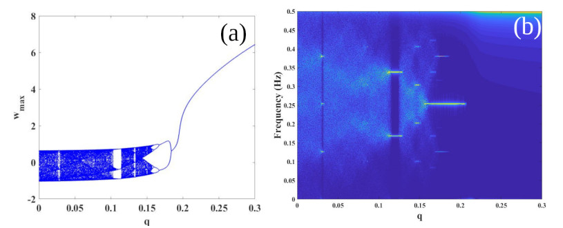
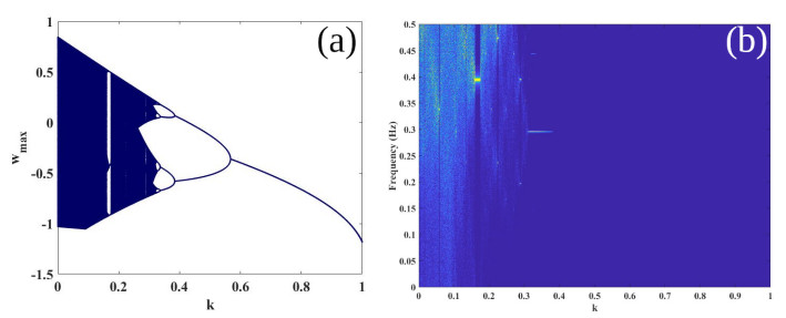
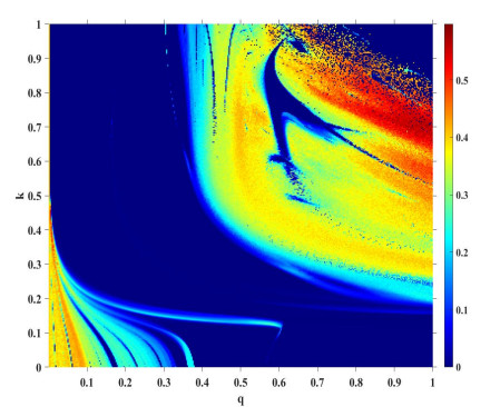
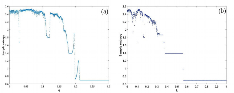
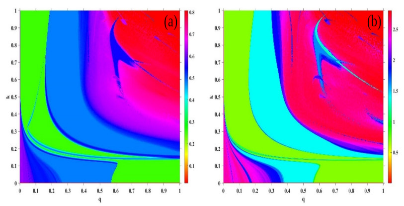
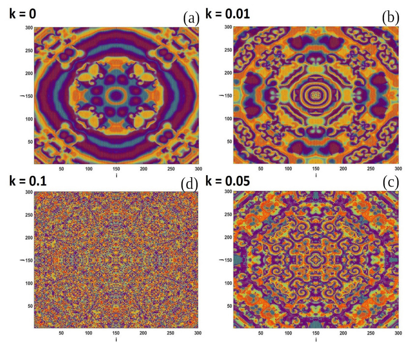
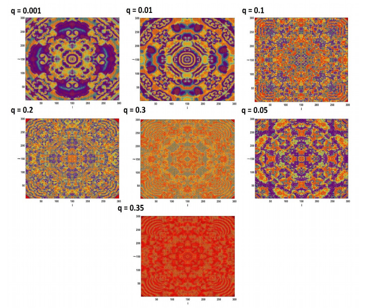
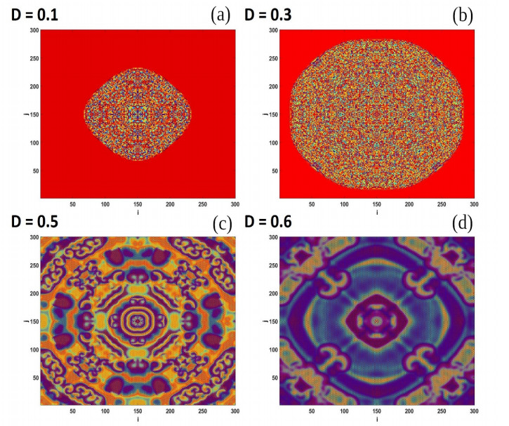
We discuss the dynamics of a fractional order discrete neuron model with electromagnetic flux coupling. The discussed neuron model is a simple one-dimensional map which is modified by considering flux coupling. We consider a discrete fractional order memristor to mimic the effects of electromagnetic flux on the neuron model. The bifurcation dynamics of the fractional order neuron map show an inverse period-doubling route to chaos as a function of control parameters, namely the fractional order of the map and the flux coupling coefficient. The bifurcation dynamics of the systems are derived both in the time and frequency domains. We present a two-parameter phase diagram using the Lyapunov exponent to categorize the various dynamics present in the system. In addition to the Lyapunov exponent, we use the entropy of the model to distinguish the various dynamics of the systems. To investigate the network behavior of the fractional order neuron map, a lattice array of $ N\times N $ nodes is constructed and external periodic stimuli are applied to the network. The formation of spiral waves in the network and the impact of various parameters, like the fractional order, flux coupling coefficient and the coupling strength on the wave propagation are also considered in our analysis.
Citation: Janarthanan Ramadoss, Asma Alharbi, Karthikeyan Rajagopal, Salah Boulaaras. A fractional-order discrete memristor neuron model: Nodal and network dynamics[J]. Electronic Research Archive, 2022, 30(11): 3977-3992. doi: 10.3934/era.2022202
We discuss the dynamics of a fractional order discrete neuron model with electromagnetic flux coupling. The discussed neuron model is a simple one-dimensional map which is modified by considering flux coupling. We consider a discrete fractional order memristor to mimic the effects of electromagnetic flux on the neuron model. The bifurcation dynamics of the fractional order neuron map show an inverse period-doubling route to chaos as a function of control parameters, namely the fractional order of the map and the flux coupling coefficient. The bifurcation dynamics of the systems are derived both in the time and frequency domains. We present a two-parameter phase diagram using the Lyapunov exponent to categorize the various dynamics present in the system. In addition to the Lyapunov exponent, we use the entropy of the model to distinguish the various dynamics of the systems. To investigate the network behavior of the fractional order neuron map, a lattice array of $ N\times N $ nodes is constructed and external periodic stimuli are applied to the network. The formation of spiral waves in the network and the impact of various parameters, like the fractional order, flux coupling coefficient and the coupling strength on the wave propagation are also considered in our analysis.

| [1] | I. Podlubny, Fractional Differential Equations: An Introduction to Fractional Derivatives, Academic Press, 1998. |
| [2] |
H. Liu, S. Li, J. Cao, G, Li, A. Alsaedi, F. E. Alsaadi, Adaptive fuzzy prescribed performance controller design for a class of uncertain fractional-order nonlinear systems with external disturbances, Neurocomputing, 219 (2017), 422–430. https://doi.org/10.1016/j.neucom.2016.09.050 doi: 10.1016/j.neucom.2016.09.050

|
| [3] |
H. Wu, L. Wang, Y. Wang, P. Niu, B. Fang, Global Mittag-Leffler projective synchronization for fractional-order neural networks: an LMI-based approach, Adv. Differ. Equations, 132 (2016), 1–18. https://doi.org/10.1186/s13662-016-0857-8 doi: 10.1186/s13662-016-0857-8
|
| [4] | A. A. Kilbas, H. M. Srivastava, J. J. Trujillo, Theory and applications of fractional differential equations, Elsevier Science, 2006. |
| [5] |
J. S. Jacob, J. H. Priya, A. Karthika, Applications of fractional calculus in science and engineering, J. Crit. Rev., 7 (2020), 4385–4394. https://doi.org/10.31838/jcr.07.13.670 doi: 10.31838/jcr.07.13.670
|
| [6] | E. Kaslik, S. Sivasundaram, Dynamics of fractional-order neural networks, in The 2011 International Joint Conference on Neural Networks, 2011. |
| [7] |
L. Si, M. Xiao, G. Jiang, Z. Cheng, Q. Song, J. Cao, Dynamics of fractional-order neural networks with discrete and distributed delays, IEEE Access, 8 (2019), 46071–46080. https://doi.org/10.1109/ACCESS.2019.2946790 doi: 10.1109/ACCESS.2019.2946790
|
| [8] |
H. Meneses, E. Guevara, O. Arrieta, F. Padula, R. Vilanova, A. Visioli, Improvement of the control system performance based on fractional-order PID controllers and models with robustness considerations, IFAC-PapersOnLine, 51 (2018), 551–556. https://doi.org/10.1016/j.ifacol.2018.06.153 doi: 10.1016/j.ifacol.2018.06.153
|
| [9] |
M. M. Al-sawalha, Synchronization of different order fractional-order chaotic systems using modify adaptive sliding mode control, Adv. Differ. Equations, 2020 (2020), 1–17. https://doi.org/10.1186/s13662-020-02876-7 doi: 10.1186/s13662-020-02876-7
|
| [10] |
S. He, H. Natiq, S. Banerjee, K. Sun, Complexity and Chimera States in a network of fractional-order Laser systems, Symmetry, 13 (2021), 341. https://doi.org/10.3390/sym13020341 doi: 10.3390/sym13020341
|
| [11] |
H. Fan, Y. Zhao, Cluster synchronization of fractional-order nonlinearly-coupling community networks with time-varying disturbances and multiple delays, IEEE Access, 9, (2021), 60934–60945. https://doi.org/10.1109/ACCESS.2021.3074016 doi: 10.1109/ACCESS.2021.3074016
|
| [12] |
W. Zhang, J. Cao, D. Chen, F. E. Alsaadi, Synchronization in fractional-order complex-valued delayed neural networks, Entropy, 20 (2018), 54. https://doi.org/10.3390/e20010054 doi: 10.3390/e20010054
|
| [13] |
H. Bao, J. H. Park, J. Cao, Adaptive synchronization of fractional-order memristor-based neural networks with time delay, Nonlinear Dyn., 82 (2015), 1343–1354. https://doi.org/10.1007/s11071-015-2242-7 doi: 10.1007/s11071-015-2242-7
|
| [14] | X. Yang, G. Zhang, X. Li, D. Wang, The synchronization and synchronization transition of coupled fractional-order neuronal networks, preprint. https://doi.org/10.21203/rs.3.rs-458795/v1 |
| [15] |
P. Vázquez-Guerrero, J. F. Gómez-Aguilar, F. Santamaria, R. F. Escobar Jiménez, Design of a high-gain observer for the synchronization of chimera states in neurons coupled with fractional dynamics, Phys. A: Stat. Mech. Appl., 539 (2020), 122896. https://doi.org/10.1016/j.physa.2019.122896 doi: 10.1016/j.physa.2019.122896
|
| [16] |
P. Vázquez-Guerrero, J. F. Gómez-Aguilar, F. Santamaria, R. F. Escobar Jiménez, Synchronization patterns with strong memory adaptive control in networks of coupled neurons with chimera states dynamics, Chaos Solitons Fractals, 128 (2019), 167–175. https://doi.org/10.1016/j.chaos.2019.07.057 doi: 10.1016/j.chaos.2019.07.057
|
| [17] |
S. He, Complexity and chimera states in a ring-coupled fractional-order memristor neural network, Front. Appl. Math. Stat., 6 (2020), 24. https://doi.org/10.3389/fams.2020.00024 doi: 10.3389/fams.2020.00024
|
| [18] |
J. Ramadoss, S. Aghababaei, F. Parastesh, K. Rajagopal, S. Jafari, I. Hussain, Chimera state in the network of fractional-order Fitzhugh–Nagumo neurons, Complexity, 2021 (2021), 9. https://doi.org/10.1155/2021/2437737 doi: 10.1155/2021/2437737
|
| [19] |
Y. Xu, J. Liu, W. Li, Quasi-synchronization of fractional-order multi-layer networks with mismatched parameters via delay-dependent impulsive feedback control, Neural Networks, 150 (2022), 43–57. https://doi.org/10.1016/j.neunet.2022.02.023 doi: 10.1016/j.neunet.2022.02.023
|
| [20] |
H. Zhang, J. Cheng, H. Zhang, W. Zhang, J. Cao, Quasi-uniform synchronization of Caputo type fractional neural networks with leakage and discrete delays, Chaos Solitons Fractals, 152 (2021), 111432. https://doi.org/10.1016/j.chaos.2021.111432 doi: 10.1016/j.chaos.2021.111432
|
| [21] |
H. Zhang, Y. Cheng, H. Zhang, W. Zhang, J. Cao, Hybrid control design for Mittag-Leffler projective synchronization on FOQVNNs with multiple mixed delays and impulsive effects, Math. Comput. Simul., 197 (2022), 341–357. https://doi.org/10.1016/j.matcom.2022.02.022 doi: 10.1016/j.matcom.2022.02.022
|
| [22] |
Y. Xu, S. Gao, W. Li, Exponential stability of fractional-order complex multi-links networks with aperiodically intermittent control, IEEE Trans. Neural Networks Learning Syst., 32 (2020), 4063–4074. https://doi.org/10.1109/TNNLS.2020.3016672 doi: 10.1109/TNNLS.2020.3016672
|
| [23] |
V. Varshney, S. Kumarasamy, A. Mishra, B. Biswal, A. Prasad, Traveling of extreme events in network of counter-rotating nonlinear oscillators, Chaos Int. J. Nonlinear Sci., 31 (2021), 093136. https://doi.org/10.1063/5.0059750 doi: 10.1063/5.0059750
|
| [24] |
Z. Rostami, S. Jafari, Defects formation and spiral waves in a network of neurons in presence of electromagnetic induction, Cognit. Neurondyn., 12 (2018), 235–254. https://doi.org/10.1007/s11571-017-9472-y doi: 10.1007/s11571-017-9472-y
|
| [25] |
A. R. Nayak, A. V. Panfilov, R. Pandit, Spiral-wave dynamics in a mathematical model of human ventricular tissue with myocytes and Purkinje fibers, Phy. Rev. E, 95 (2017), 022405. https://doi.org/10.1103/PhysRevE.95.022405 doi: 10.1103/PhysRevE.95.022405
|
| [26] |
V. Petrov, Q. Ouyang, H. L. Swinney, Resonant pattern formation in a chemical system, Nature, 388 (1997), 655–657. https://doi.org/10.1038/41732 doi: 10.1038/41732
|
| [27] |
S. Woo, J. Lee, K. J. Lee, Spiral waves in a coupled network of sine-circle maps, Phys. Rev. E, 68 (2003), 016208. https://doi.org/10.1103/PhysRevE.68.016208 doi: 10.1103/PhysRevE.68.016208
|
| [28] |
A. Bukh, G. Strelkova, V. Anishchenko, Spiral wave patterns in a two-dimensional lattice of nonlocally coupled maps modeling neural activity, Chaos Solitons Fractals, 120 (2019), 75–82. https://doi.org/10.1016/j.chaos.2018.11.037 doi: 10.1016/j.chaos.2018.11.037
|
| [29] |
Y. Feng, A. J. M. Khalaf, F. E. Alsaadi, T. Hayat, V. Pham, Spiral wave in a two-layer neuronal network, Eur. Phys. Spec. Top., 228 (2019), 2371–2379. https://doi.org/10.1140/epjst/e2019-900082-6 doi: 10.1140/epjst/e2019-900082-6
|
| [30] |
K. Rajagopal, S. Jafari, I. Moroz, A. Karthikeyan, A. Srinivasan, Noise induced suppression of spiral waves in a hybrid FitzHugh–Nagumo neuron with discontinuous resetting, Chaos, 31 (2021), 073117. https://doi.org/10.1063/5.0059175 doi: 10.1063/5.0059175
|
| [31] |
K. Aihara, T. Takabe, M. Toyoda, Chaotic neural networks, Phys. Lett. A, 144 (1990), 333–340. https://doi.org/10.1016/0375-9601(90)90136-C doi: 10.1016/0375-9601(90)90136-C
|
| [32] |
J. Nagumo, S. Sato, On a response characteristic of a mathematical neuron model, Kybernetik, 10 (1972), 155–164. https://doi.org/10.1007/BF00290514 doi: 10.1007/BF00290514
|
| [33] |
S. Momani, A. Freihat, M. AL-Smadi, Analytical study of fractional-order multiple chaotic Fitzhugh-Nagumo neurons model using multistep generalized differential transform method, Abstract Appl. Anal., 2014 (2014), 10. https://doi.org/10.1155/2014/276279 doi: 10.1155/2014/276279
|
| [34] |
Y. Peng, K. Sun, S. He, A discrete memristor model and its application in Hénon map, Chaos Solitons Fractals, 137 (2021), 109873. https://doi.org/10.1016/j.chaos.2020.109873 doi: 10.1016/j.chaos.2020.109873
|
| [35] |
Y. Deng, Y. Li, Bifurcation and bursting oscillations in 2D non-autonomous discrete memristor-based hyperchaotic map, Chaos Solitons Fractals, 150 (2021), 111064. https://doi.org/10.1016/j.chaos.2021.111064 doi: 10.1016/j.chaos.2021.111064
|
| [36] |
L. Montesinos, R. Castaldo, L. Pecchia, On the use of approximate entropy and sample entropy with centre of pressure time-series, J. NeuroEng. Rehabil., 15 (2018), 116. https://doi.org/10.1186/s12984-018-0465-9 doi: 10.1186/s12984-018-0465-9
|
| [37] |
J. Palanivel, K. Suresh, D. Premraj, K. Thamilmaran, Effect of fractional-order, time-delay and noisy parameter on slow-passage phenomenon in a nonlinear oscillator, Chaos Solitons Fractals, 106 (2018), 35–43. https://doi.org/10.1016/j.chaos.2017.11.006 doi: 10.1016/j.chaos.2017.11.006
|
| [38] |
J. Palanivel, K. Suresh, S. Sabarathinam, K. Thamilmaran, Chaos in a low dimensional fractional-order nonautonomous nonlinear oscillator, Chaos Solitons Fractals, 95 (2017), 33–41. https://doi.org/10.1016/j.chaos.2016.12.007 doi: 10.1016/j.chaos.2016.12.007
|
Figures(8)
Janarthanan Ramadoss, Asma Alharbi, Karthikeyan Rajagopal, Salah Boulaaras. A fractional-order discrete memristor neuron model: Nodal and network dynamics[J]. Electronic Research Archive, 2022, 30(11): 3977-3992. doi: 10.3934/era.2022202


 DownLoad: