The detection of neurological disorders and diseases is aided by automatically identifying brain tumors from brain magnetic resonance imaging (MRI) images. A brain tumor is a potentially fatal disease that affects humans. Convolutional neural networks (CNNs) are the most common and widely used deep learning techniques for brain tumor analysis and classification. In this study, we proposed a deep CNN model for automatically detecting brain tumor cells in MRI brain images. First, we preprocess the 2D brain image MRI image to generate convolutional features. The CNN network is trained on the training dataset using the GoogleNet and AlexNet architecture, and the data model's performance is evaluated on the test data set. The model's performance is measured in terms of accuracy, sensitivity, specificity, and AUC. The algorithm performance matrices of both AlexNet and GoogLeNet are compared, the accuracy of AlexNet is 98.95, GoogLeNet is 99.45 sensitivity of AlexNet is 98.4, and GoogLeNet is 99.75, so from these values, we can infer that the GooGleNet is highly accurate and parameters that GoogLeNet consumes is significantly less; that is, the depth of AlexNet is 8, and it takes 60 million parameters, and the image input size is 227 × 227. Because of its high specificity and speed, the proposed CNN model can be a competent alternative support tool for radiologists in clinical diagnosis.
Citation: Chetan Swarup, Kamred Udham Singh, Ankit Kumar, Saroj Kumar Pandey, Neeraj varshney, Teekam Singh. Brain tumor detection using CNN, AlexNet & GoogLeNet ensembling learning approaches[J]. Electronic Research Archive, 2023, 31(5): 2900-2924. doi: 10.3934/era.2023146
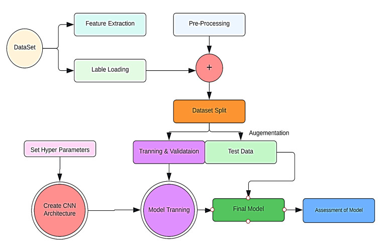
The detection of neurological disorders and diseases is aided by automatically identifying brain tumors from brain magnetic resonance imaging (MRI) images. A brain tumor is a potentially fatal disease that affects humans. Convolutional neural networks (CNNs) are the most common and widely used deep learning techniques for brain tumor analysis and classification. In this study, we proposed a deep CNN model for automatically detecting brain tumor cells in MRI brain images. First, we preprocess the 2D brain image MRI image to generate convolutional features. The CNN network is trained on the training dataset using the GoogleNet and AlexNet architecture, and the data model's performance is evaluated on the test data set. The model's performance is measured in terms of accuracy, sensitivity, specificity, and AUC. The algorithm performance matrices of both AlexNet and GoogLeNet are compared, the accuracy of AlexNet is 98.95, GoogLeNet is 99.45 sensitivity of AlexNet is 98.4, and GoogLeNet is 99.75, so from these values, we can infer that the GooGleNet is highly accurate and parameters that GoogLeNet consumes is significantly less; that is, the depth of AlexNet is 8, and it takes 60 million parameters, and the image input size is 227 × 227. Because of its high specificity and speed, the proposed CNN model can be a competent alternative support tool for radiologists in clinical diagnosis.

| [1] |
F. Abdolkarimzadeh, M. R. Ashory, A. Ghasemi-Ghalebahman, A. Karimi, Inverse dynamic finite element-optimization modeling of the brain tumor mass-effect using a variable pressure boundary, Comput. Methods Programs Biomed., 212 (2021), 106476, https://doi.org/10.1016/j.cmpb.2021.106476 doi: 10.1016/j.cmpb.2021.106476

|
| [2] |
R. R. Agravat, M. S. Raval, A survey and analysis on automated glioma brain tumor segmentation and overall patient survival prediction, Arch. Comput. Methods Eng., 28 (2021), 4117–4152. https://doi.org/10.1007/s11831-021-09559-w doi: 10.1007/s11831-021-09559-w
|
| [3] |
A. M. Alhassan, W. Zainon, Brain tumor classification in magnetic resonance image using hard swish-based RELU activation function-convolutional neural network, Neural Comput. Appl., 33 (2021), 9075–9087. https://doi.org/10.1007/s00521-020-05671-3 doi: 10.1007/s00521-020-05671-3
|
| [4] |
M. Alshayeji, J. Al-Buloushi, A. Ashkanani, S. Abed, Enhanced brain tumor classification using an optimized multi-layered convolutional neural network architecture, Multimedia Tools Appl., 80 (2021), 28897–28917. https://doi.org/10.1007/s11042-021-10927-8 doi: 10.1007/s11042-021-10927-8
|
| [5] |
W. Ayadi, W. Elhamzi, I. Charfi, M. Atri, Deep CNN for brain tumor classification, Neural Process. Lett., 53 (2021), 671–700. https://doi.org/10.1007/s11063-020-10398-2 doi: 10.1007/s11063-020-10398-2
|
| [6] |
F. Bashir-Gonbadi, H. Khotanlou, Brain tumor classification using deep convolutional autoencoder-based neural network: Multi-task approach, Multimed. Tools Appl., 80 (2021), 19909–19929. https://doi.org/10.1007/s11042-021-10637-1 doi: 10.1007/s11042-021-10637-1
|
| [7] |
B. S. Chen, L. L. Zhang, H. Y. Chen, K. W. Liang, X. Z. Chen, A novel extended Kalman filter with support vector machine based method for the automatic diagnosis and segmentation of brain tumors, Comput. Methods Prog. Biomed., 200 (2021), 105797. https://doi.org/10.1016/j.cmpb.2020.105797 doi: 10.1016/j.cmpb.2020.105797
|
| [8] |
N. V. Dhole, V. V. Dixit, Review of brain tumor detection from MRI images with hybrid approaches, Multimed. Tools Appl., 81 (2022), 10189–10220. https://doi.org/10.1007/s11042-022-12162-1 doi: 10.1007/s11042-022-12162-1
|
| [9] |
B. V. Isunuri, J. Kakarla, Three-class brain tumor classification from magnetic resonance images using separable convolution based neural network, Concurr. Comput. Prac. Experience, 34 (2022), e6541–e6549. https://doi.org/10.1002/cpe.6541 doi: 10.1002/cpe.6541
|
| [10] |
T. A. Jemimma, Y. J. V. Raj, Significant LOOP with clustering approach and optimization enabled deep learning classifier for the brain tumor segmentation and classification, Multimed. Tools Appl., 81 (2022), 2365–2391. https://doi.org/10.1007/s11042-021-11591-8 doi: 10.1007/s11042-021-11591-8
|
| [11] |
B. Jena, G. K. Nayak, S. Saxena, An empirical study of different machine learning techniques for brain tumor classification and subsequent segmentation using hybrid texture feature, Mach. Vision Appl., 33 (2022), 1–16. https://doi.org/10.1007/s00138-021-01262-x doi: 10.1007/s00138-021-01262-x
|
| [12] |
M. Jiang, F. H. Zhai, J. Kong, A novel deep learning model DDU-net using edge features to enhance brain tumor segmentation on MR images, Artif. Intell. Med., 121 (2021), 102180. https://doi.org/10.1016/j.artmed.2021.102180 doi: 10.1016/j.artmed.2021.102180
|
| [13] |
S. Kadry, V. Rajinikanth, N. S. M. Raja, D. J. Hemanth, N. M. S. Hannon, A. N. J. Raj, Evaluation of brain tumor using brain MRI with modified-moth-flame algorithm and Kapu's thresholding: A study, Evol. Intell., 14 (2021), 1053–1063. https://doi.org/10.1007/s12065-020-00539-w doi: 10.1007/s12065-020-00539-w
|
| [14] |
S. Kokkalla, J. Kakarla, I. B. Venkateswarlu, M. Singh, Three-class brain tumor classification using deep dense inception residual network, Soft Comput., 25 (2021), 8721–8729. https://doi.org/10.1007/s00500-021-05748-8 doi: 10.1007/s00500-021-05748-8
|
| [15] |
R. L. Kumar, J. Kakarla, B. V. Isunuri, M. Singh, Multiclass brain tumor classification using residual network and global average pooling, Multimed. Tools Appl., 80 (2021), 13429–13438. https://doi.org/10.1007/s11042-020-10335-4 doi: 10.1007/s11042-020-10335-4
|
| [16] |
Y. Guan, M. Aamir, Z. Rahman, A. Ali, W. A. Abro, Z. A. Dayo, et al., A framework for efficient brain tumor classification using MRI images, Math. Biosci. Eng., 18 (2021), 5790–5815. https://doi.org/10.3934/mbe.2021292 doi: 10.3934/mbe.2021292
|
| [17] |
M. Aamir, Z. Rahman, Z. A. Dayo, W. A. Abro, M. I. Uddin, I. Khan, et al., A deep learning approach for brain tumour classification using MRI images, Comput. Electr. Eng., 101 (2022), 108105. https://doi.org/10.1016/j.compeleceng.2022.108105 doi: 10.1016/j.compeleceng.2022.108105
|
| [18] |
X. L. Lei, X. S. Yu, J. N. Chi, Y. Wang, J. S. Zhang, C. D. Wu, Brain tumor segmentation in MR images using a sparse constrained level set algorithm, Expert Syst. Appl., 168 (2021), 114262. https://doi.org/10.1016/j.eswa.2020.114262 doi: 10.1016/j.eswa.2020.114262
|
| [19] |
G. L. Li, J. H. Sun, Y. L. Song, J. F. Qu, Z. Y. Zhu, M. R. Khosravi, Real-time classification of brain tumors in MRI images with a convolutional operator-based hidden Markov model, J. Real Time Image Process., 18 (2021), 1207–1219. https://doi.org/10.1007/s11554-021-01072-4 doi: 10.1007/s11554-021-01072-4
|
| [20] |
O. Polat, C. Gungen, Classification of brain tumors from MR images using deep transfer learning, J. Supercomput., 77 (2021), 7236–7252. https://doi.org/10.1007/s11227-020-03572-9 doi: 10.1007/s11227-020-03572-9
|
| [21] |
S. Preethi, P. Aishwarya, An efficient wavelet-based image fusion for brain tumor detection and segmentation over PET and MRI image, Multimed. Tools Appl., 80 (2021), 14789–14806. https://doi.org/10.1007/s11042-021-10538-3 doi: 10.1007/s11042-021-10538-3
|
| [22] |
S. Ramesh, S. Sasikala, N. Paramanandham, Segmentation and classification of brain tumors using modified median noise filter and deep learning approaches, Multimed. Tools Appl., 80 (2021), 11789–11813. https://doi.org/10.1007/s11042-020-10351-4 doi: 10.1007/s11042-020-10351-4
|
| [23] |
C. S. Rao, K. Karunakara, A comprehensive review on brain tumor segmentation and classification of MRI images, Multimed. Tools Appl., 80 (2021), 17611–17643. https://doi.org/10.1007/s11042-020-10443-1 doi: 10.1007/s11042-020-10443-1
|
| [24] |
A. S. Reddy, P. C. Reddy, MRI brain tumor segmentation and prediction using modified region growing and adaptive SVM, Soft Comput., 25 (2021), 4135–4148. https://doi.org/10.1007/s00500-020-05493-4 doi: 10.1007/s00500-020-05493-4
|
| [25] |
V. V. S. Sasank, S. Venkateswarlu, Brain tumor classification using modified kernel based softplus extreme learning machine, Multimed. Tools Appl., 80 (2021), 3513–13534. https://doi.org/10.1007/s11042-020-10423-5 doi: 10.1007/s11042-020-10423-5
|
| [26] |
V. V. S. Sasank, S. Venkateswarlu, Hybrid deep neural network with adaptive rain optimizer algorithm for multi-grade brain tumor classification of MRI images, Multimed. Tools Appl., 81 (2022), 8021–8057. https://doi.org/10.1007/s11042-022-12106-9 doi: 10.1007/s11042-022-12106-9
|
| [27] |
S. N. Shivhare, N. Kumar, Tumor bagging: A novel framework for brain tumor segmentation using metaheuristic optimization algorithms, Multimed. Tools Appl., 80 (2021), 26969–26995. https://doi.org/10.1007/s11042-021-10969-y doi: 10.1007/s11042-021-10969-y
|
| [28] |
J. J. Wang, J. Gao, J. Ren, Z. Luan, Z. Yu, Y. Zhao, et al., DFP-ResUNet: Convolutional neural network with a dilated convolutional feature pyramid for multimodal brain tumor segmentation, Comput. Methods Prog. Biomed., 208 (2021), 106208. https://doi.org/10.1016/j.cmpb.2021.106208 doi: 10.1016/j.cmpb.2021.106208
|
| [29] |
P. Wang, A. C. S. Chung, Relax and focus on brain tumor segmentation, Medical Image Anal., 75 (2022), 102259. https://doi.org/10.1016/j.media.2021.102259 doi: 10.1016/j.media.2021.102259
|
| [30] |
Y. Wang, J. L. Peng, Z. D. Jia, Brain tumor segmentation via C-dense convolutional neural network, Prog. Artif. Intell., 10 (2021), 147–156. https://doi.org/10.1007/s13748-021-00232-8 doi: 10.1007/s13748-021-00232-8
|
| [31] |
Y. L. Wang, Z. J. Zhao, S. Y. Hu, F. L. Chang, CLCU-Net: Cross-level connecte d U-shape d network with selective feature aggregation attention module for brain tumor segmentation, Comput. Methods Prog Biomed., 207 (2021), 106154. https://doi.org/10.1016/j.cmpb.2021.106154 doi: 10.1016/j.cmpb.2021.106154
|
| [32] |
X. H. Wu, L. Bi, M. Fulham, D. D. Feng, L. P. Zhou, and J. Kim, Unsupervised brain tumor segmentation using a symmetric-driven adversarial network, Neurocomputing, 455 (2021), 242–254. https://doi.org/10.1016/j.neucom.2021.05.073 doi: 10.1016/j.neucom.2021.05.073
|
| [33] |
D. W. Zhang, G. H. Huang, Q. Zhang, J. G. Han, J. W. Han, Y. Z. Yu, Cross-modality deep feature learning for brain tumor segmentation, Pattern Recogn., 110 (2021), 107562. https://doi.org/10.1016/j.patcog.2020.107562 doi: 10.1016/j.patcog.2020.107562
|
| [34] |
H. ZainEldin, S. A. Gamel, E. M. El-Kenawy, A. H. Alharbi, D. S. Khafaga, A. Ibrahim, et al., Brain tumor detection and classification using deep learning and sine-cosine fitness grey wolf optimization, Bioengineering, 1 (2023), 10–18. https://doi.org/10.3390/bioengineering10010018 doi: 10.3390/bioengineering10010018
|
| [35] | V. Kushwaha, P. Maidamwar, BTFCNN: Design of a brain tumor classification model using fused convolutional neural networks, in 2022 10th International Conference on Emerging Trends in Engineering and Technology-Signal and Information Processing (ICETET-SIP-22), (2022), 1–6. https://doi.org/10.1109/ICETET-SIP-2254415.2022.9791734 |
| [36] |
Y. Guan, M. Aamir, Z. Rahman, A. Ali, W. A. Abro, Z. A. Dayo, et al., A framework for efficient brain tumor classification using MRI images, Math. Biosci. Eng., 18 (2021), 5790–5815. https://doi.org/10.3934/mbe.2021292 doi: 10.3934/mbe.2021292
|
| [37] |
M. Aamir, Z. Rahman, Z. A. Dayo, W. A. Abro, M. I. Uddin, I. Khan, et al., A deep learning approach for brain tumour classification using MRI images, Comput. Electr. Eng., 1 (2022), 108105–108120. https://doi.org/10.1016/j.compeleceng.2022.108105 doi: 10.1016/j.compeleceng.2022.108105
|
| [38] |
M. M. Badža, M. Č. Barjaktarović, Classification of brain tumors from MRI images using a convolutional neural network., Appl. Sci. (Basel), 10 (2020), 1999–2020. https://doi.org/10.3390/app10061999 doi: 10.3390/app10061999
|
| [39] |
N. Zheng, G. Zhang, Y. Zhang, F. R. Sheykhahmad, Brain tumor diagnosis based on Zernike moments and support vector machine optimized by chaotic arithmetic optimization algorithm, Biomed. Signal Process. Control., 82 (2023), 104543, 104543–104553. https://doi.org/10.1016/j.bspc.2022.104543 doi: 10.1016/j.bspc.2022.104543
|
| [40] |
Q. Zhou, Medical image classification using light-weight CNN with spiking cortical model based attention module, IEEE J. Biomed. Health Inform., 1 (2023), 1–13. https://doi.org/10.1109/JBHI.2023.3241439 doi: 10.1109/JBHI.2023.3241439
|
| [41] |
S. Deepak, P. M. Ameer, Brain tumor categorization from imbalanced MRI dataset using weighted loss and deep feature fusion, Neurocomputing, 520 (2023), 94–102. https://doi.org/10.1016/j.neucom.2022.11.039 doi: 10.1016/j.neucom.2022.11.039
|
| [42] |
G. Xiao, H. Wang, J. Shen, Z. Chen, Z. Zhang, X. Ge, Contrastive learning with dynamic weighting and jigsaw augmentation for brain tumor classification in mrI, Neural Process Lett., 1 (2023), 1–29. https://doi.org/10.1007/s11063-022-11108-w doi: 10.1007/s11063-022-11108-w
|


Figures(12) / Tables(8)
Chetan Swarup, Kamred Udham Singh, Ankit Kumar, Saroj Kumar Pandey, Neeraj varshney, Teekam Singh. Brain tumor detection using CNN, AlexNet & GoogLeNet ensembling learning approaches[J]. Electronic Research Archive, 2023, 31(5): 2900-2924. doi: 10.3934/era.2023146


 DownLoad: