Stability analysis of time-delayed SAIR model for duration of vaccine in the context of temporary immunity for COVID-19 situation

Zimeng Lv; Jiahong Zeng; Yuting Ding; Xinyu Liu; Zimeng Lv; Jiahong Zeng; Yuting Ding; Xinyu Liu

doi:10.3934/era.2023050

Electronic Research Archive

2023, Volume 31, Issue 2: 1004-1030. doi: 10.3934/era.2023050

Previous Article Next Article

Theory article Special Issues

Stability analysis of time-delayed SAIR model for duration of vaccine in the context of temporary immunity for COVID-19 situation

College of Science, Northeast Forestry University, Harbin 150040, China

Received: 30 September 2022 Revised: 04 December 2022 Accepted: 06 December 2022 Published: 09 December 2022

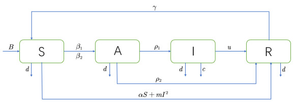
As the COVID-19 continues threatening public health worldwide, when to vaccinate the booster shots becomes the hot topic. In this paper, based on the characteristics of COVID-19 and its vaccine, an $ SAIR $ model associated with temporary immunity is proposed to study the effect on epidemic situation. Second, we theoretically analyze the existence and stability of equilibrium and the system undergoes Hopf bifurcation when delay passes through some critical values. Third, we study the dynamic properties of Hopf bifurcation and derive the normal form of Hopf bifurcation to determine the stability and direction of bifurcating periodic solutions. After that, numerical simulations are carried out to demonstrate the application of the theoretical results. Particularly, in order to ensure the validity, statistical analysis of data is conducted to determine the values for model parameters. Next, we study the impact of the infection rates on booster vaccination time to simulate the mutants, and the results are consistent with the facts. Finally, we predict the mean time of completing a round of vaccination worldwide with the help fitting and put forward some suggestions by comparing with the critical time of booster vaccination.
- SARS-CoV-2019,
- booster vaccination,
- stability,
- time delay,
- Hopf bifurcation
Citation: Zimeng Lv, Jiahong Zeng, Yuting Ding, Xinyu Liu. Stability analysis of time-delayed SAIR model for duration of vaccine in the context of temporary immunity for COVID-19 situation[J]. Electronic Research Archive, 2023, 31(2): 1004-1030. doi: 10.3934/era.2023050

Related Papers:

Abstract

As the COVID-19 continues threatening public health worldwide, when to vaccinate the booster shots becomes the hot topic. In this paper, based on the characteristics of COVID-19 and its vaccine, an $ SAIR $ model associated with temporary immunity is proposed to study the effect on epidemic situation. Second, we theoretically analyze the existence and stability of equilibrium and the system undergoes Hopf bifurcation when delay passes through some critical values. Third, we study the dynamic properties of Hopf bifurcation and derive the normal form of Hopf bifurcation to determine the stability and direction of bifurcating periodic solutions. After that, numerical simulations are carried out to demonstrate the application of the theoretical results. Particularly, in order to ensure the validity, statistical analysis of data is conducted to determine the values for model parameters. Next, we study the impact of the infection rates on booster vaccination time to simulate the mutants, and the results are consistent with the facts. Finally, we predict the mean time of completing a round of vaccination worldwide with the help fitting and put forward some suggestions by comparing with the critical time of booster vaccination.

References

[1]	E. Petersen, M. Koopmans, U. Go, D. H. Hamer, N. Petrosillo, F. Castelli, et al., Comparing SARS-CoV-2 with SARS-CoV and influenza pandemics, Lancet Infect. Dis., 20 (2020), e238–e244. https://doi.org/10.1016/S1473-3099(20)30484-9 doi: 10.1016/S1473-3099(20)30484-9
[2]	B. A. Connor, M. Couto-Rodriguez, J. E. Barrows, M. Rodriguez, M. Rogova, N. B. O'Hara, et al., Monoclonal antibody therapy in a vaccine breakthrough SARS-CoV-2 hospitalized Delta (B.1.617.2) variant case, Int. J. Infect. Dis., 110 (2021), 232–234. https://doi.org/10.1016/j.ijid.2021.07.029 doi: 10.1016/j.ijid.2021.07.029
[3]	A. Din, Y. Li, A. Yusuf, A. I. Alt, Caputo type fractional operator applied to Hepatitis B system, Fractals, 30 (2022), 2240023. https://doi.org/10.1142/S0218348X22400230 doi: 10.1142/S0218348X22400230
[4]	A. Din, Y. Li, F. M. Khan, Z. U. Khan, P. Liu, On Analysis of fractional order mathematical model of Hepatitis B using Atangana Baleanu Caputo (ABC) derivative, Fractals, 30 (2022), 2240017. https://doi.org/10.1142/S0218348X22400175 doi: 10.1142/S0218348X22400175
[5]	P. Liu, A. Din, Zenab, Impact of information intervention on stochastic dengue epidemic model, Alexandria Eng. J., 60 (2021), 5725–5739. https://doi.org/10.1016/j.aej.2021.03.068 doi: 10.1016/j.aej.2021.03.068
[6]	A. Din, Y. Li, T. Khan, G. Zaman, Mathematical analysis of spread and control of the novel corona virus (COVID-19) in China, Chaos, Solitons Fractals, 141 (2020), 110286. https://doi.org/10.1016/j.chaos.2020.110286 doi: 10.1016/j.chaos.2020.110286
[7]	J. Arino, F. Brauer, P. van den Driessche, J. Watmough, J. Wu, A model for influenza with vaccination and antiviral treatment, J. Theor. Biol., 253 (2008), 118–130. https://doi.org/10.1016/j.jtbi.2008.02.026 doi: 10.1016/j.jtbi.2008.02.026
[8]	D. Greenhalgh, Q. J. A. Khan, F. I. Lewis, Recurrent epidemic cycles in an infectious disease model with a time delay in loss of vaccine immunity, Nonlinear Anal., 63 (2005), e779–e788. https://doi.org/10.1016/j.na.2004.12.018 doi: 10.1016/j.na.2004.12.018
[9]	B. Ho, K. Chao, On the influenza vaccination policy through mathematical modeling, Int. J. Infect. Dis., 98 (2020), 71–79. https://doi.org/10.1016/j.ijid.2020.06.043 doi: 10.1016/j.ijid.2020.06.043
[10]	S. Djilali, S. Bentout, Global dynamics of SVIR epidemic model with distributed delay and imperfect vaccine, Results Phys., 25 (2021), 104245. https://doi.org/10.1016/j.rinp.2021.104245 doi: 10.1016/j.rinp.2021.104245
[11]	K. M. A. Kabir, J. Tanimoto, A cyclic epidemic vaccination model: Embedding the attitude of individuals toward vaccination into SVIS dynamics through social interactions, Physica, 581 (2021), 126230. https://doi.org/10.1016/j.physa.2021.126230 doi: 10.1016/j.physa.2021.126230
[12]	V. Ram, L. P. Schaposnik, A modified age-structured SIR model for COVID-19 type viruses, Sci. Rep., 11 (2021), 15194. https://doi.org/10.1038/s41598-021-94609-3 doi: 10.1038/s41598-021-94609-3
[13]	M. Shen, J. Zu, C. K. Fairley, J. A. Pagïn, L. An, Z. Du, et al., Projected COVID-19 epidemic in the United States in the context of theeffectiveness of a potential vaccine and implications for social distancingand face mask use, Vaccine, 39 (2021), 2295–2302. https://doi.org/10.1016/j.vaccine.2021.02.056 doi: 10.1016/j.vaccine.2021.02.056
[14]	A. Rajaeia, M. Raeiszadeh, V. Azimi, M. Sharifi, State estimation-based control of COVID-19 epidemic before and after vaccine development, J. Process Control, 102 (2021), 1–14. https://doi.org/10.1016/j.jprocont.2021.03.008 doi: 10.1016/j.jprocont.2021.03.008
[15]	K. L. Cooke, Stability analysis for a vector disease model, Rocky Mt. J. Math., 9 (1979), 31–41. https://doi.org/10.1216/RMJ-1979-9-1-31 doi: 10.1216/RMJ-1979-9-1-31
[16]	I. AI-Darabsah, A time-delayed SVEIR model for imperfect vaccine with a generalized nonmonotone incidence and application to measles, Appl. Math. Modell., 91 (2021), 74–92. https://doi.org/10.1016/j.apm.2020.08.084 doi: 10.1016/j.apm.2020.08.084
[17]	P. Yang, K. Wang, Dynamics for an SEIRS epidemic model with time delay on a scale-free network, Physica A, 527 (2019), 121290. https://doi.org/10.1016/j.physa.2019.121290 doi: 10.1016/j.physa.2019.121290
[18]	J. Liu, Bifurcation of a delayed SEIS epidemic model with a changing delitesbcence and nonlinear incidence rate, Discrete Dyn. Nat. Soc., 2017 (2017), 2340549. https://doi.org/10.1155/2017/2340549 doi: 10.1155/2017/2340549
[19]	Z. Zhang, S. Kundu, J. P. Tripathi, S. Bugalia, Stability and Hopf bifurcation analysis of an SVEIR epidemic model with vaccination and multiple time delays, Chaos, Solitons Fractals, 131 (2020), 109483. https://doi.org/10.1016/j.chaos.2019.109483 doi: 10.1016/j.chaos.2019.109483
[20]	A. Din, Y. Li, A. Yusuf, Delayed hepatitis B epidemic model with stochastic analysis, Chaos, Solitons Fractals, 146 (2021), 110839. https://doi.org/10.1016/j.chaos.2021.110839 doi: 10.1016/j.chaos.2021.110839
[21]	T. Kuniya, Global stability analysis with a discretization approach for an age-structured multigroup SIR epidemic model, Nonlinear Anal. Real World Appl., 12 (2011), 2640–2655. https://doi.org/10.1016/j.nonrwa.2011.03.011 doi: 10.1016/j.nonrwa.2011.03.011
[22]	X. Duan, J. Yin, X. Li, Global Hopf bifurcation of an SIRS epidemic model with age-dependent recovery, Chaos, Solitons Fractals, 104 (2017), 613–624. https://doi.org/10.1016/j.chaos.2017.09.029 doi: 10.1016/j.chaos.2017.09.029
[23]	Y. Cai, W. Wang, Stability and Hopf bifurcation of the stationary solutions to an epidemic model with cross-diffusion, Comput. Math. Appl., 70 (2015), 1906–1920. https://doi.org/10.1016/j.camwa.2015.08.003 doi: 10.1016/j.camwa.2015.08.003
[24]	Y. Zhang, J. Jia, Hopf bifurcation of an epidemic model with a nonlinear birth in population and vertical transmission, Appl. Math. Comput., 230 (2014), 164–173. https://doi.org/10.1016/j.amc.2013.12.084 doi: 10.1016/j.amc.2013.12.084
[25]	Y. Song, Y. Peng, T. Zhang, The spatially inhomogeneous Hopf bifurcation induced by memory delay in a memory-based diffusion system, J. Differ. Equations, 300 (2021), 597–624. https://doi.org/10.1016/j.jde.2021.08.010 doi: 10.1016/j.jde.2021.08.010
[26]	S. Wang, Y. Ding, H. Lu, S. Gong, Stability and bifurcation analysis of SIQR for COVID-19 epidemic model with time-delay, Math. Biosci. Eng., 18 (2021), 5505–5524. https://doi.org/10.3934/mbe.2021278 doi: 10.3934/mbe.2021278
[27]	Y. Ding, L. Zheng, Mathematical modeling and dynamics analysis of delayed nonlinear VOC emission system, Nonlinear Dyn., 109 (2022), 3157–3167. https://doi.org/10.1007/s11071-022-07532-1 doi: 10.1007/s11071-022-07532-1
[28]	Y. Ding, L. Zheng, J. Guo, Stability analysis of nonlinear glue flow system with delay, Math. Methods Appl. Sci., 30 (2022), 6861–6877. https://doi.org/10.1002/mma.8211 doi: 10.1002/mma.8211
[29]	P. van den Driessche, J. Watmough, Reproduction numbers and sub-threshold endemic equilibria for compartmental models of disease transmission, Math. Biosci., 180 (2002), 29–48. https://doi.org/10.1016/S0025-5564(02)00108-6 doi: 10.1016/S0025-5564(02)00108-6
[30]	M. D'Arienzo, A. Coniglio, Assessment of the SARS-CoV-2 basic reproduction number, $R_0$, based on the early phase of COVID-19 outbreak in Italy, Biosaf. Health, 2 (2020), 57–59. https://doi.org/10.1016/j.bsheal.2020.03.004 doi: 10.1016/j.bsheal.2020.03.004
[31]	M. Al-Marwan, The basic reproduction number of the new coronavirus pandemic with mortality for India, the Syrian Arab Republic, the United States, Yemen, China, France, Nigeria and Russia with different rate of cases, Clin. Epidemiol. Global Health, 9 (2021), 147–149. https://doi.org/10.1016/j.cegh.2020.08.005 doi: 10.1016/j.cegh.2020.08.005
[32]	Y. Wang, J. Ma, J. Cao, Basic reproduction number for the SIR epidemic in degree correlated networks, Physica D, 433 (2022), 133183. https://doi.org/10.1016/j.physd.2022.133183 doi: 10.1016/j.physd.2022.133183
[33]	X. Li, J. Wei, On the zeros of a fourth degree exponential polynomial with applications to a neural network model with delays, Chaos, Solitons Fractals, 26 (2005), 519–526. https://doi.org/10.1016/j.chaos.2005.01.019 doi: 10.1016/j.chaos.2005.01.019

Reader Comments

Your name:*

Email:*
© 2023 the Author(s), licensee AIMS Press. This is an open access article distributed under the terms of the Creative Commons Attribution License (http://creativecommons.org/licenses/by/4.0)