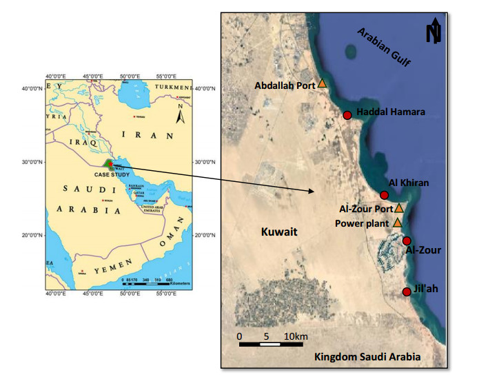
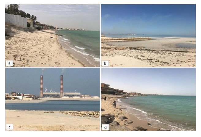
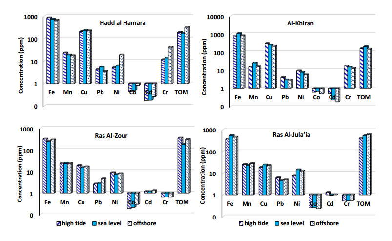
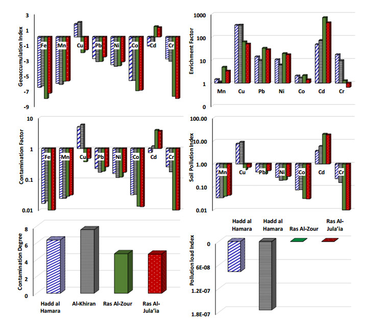
To assess the heavy metals concentration in the coastal sediments of the southern Kuwait coast, Fe, Mn, Cu, Pb, Ni, Co, Cd and Cr were measured by inductively coupled plasma mass spectroscopy. Whereas, the south of Kuwait coast is characterized by the presence of tourist resorts, and commercial and oil exports harbors. Moreover, environmental indicators were used to help in evaluating the degree and the intensity of pollutants in these sediments. Geoaccumulation index (Igeo) revealed that the sediments of hard all Hamara and Al-Khiran coasts are moderately polluted by Cu, while Ras Al-Zour and Ras Al-Jula'ia coasts are moderately polluted by Cd. Moreover, the enrichment factor (EF) indicated that the sediments of Hadd Al-Hamara coast are severely enriched with Ni, Cr and Pb, while the Al-Khiran coast is moderate severely enriched with the same metals. Ras Al-Zour and Ras Al-Jula'ia coasts are severely enriched with Ni and very severely enriched with Pb. Simultaneously, all studied sites are extremely severely enriched with Cu and Cd. These results were confirmed by the results of the contamination factor (CF) and the soil pollution index (SPI) indicated that Hadd Al-Hamara and Al-Khiran coasts are highly contaminated with Cu and Cd, while Ras Al-Zour and Ras Al-Jula'ia coasts are highly contaminated with Cd. Generally, the pollution load index showed that the sediments of all studied sites are no heavy metal pollution (PLI < 1). Pollutants might be originated from commercial wastes and construction activities.
Citation: Hamdy E. Nour, Fatma Ramadan, Nouf El Shammari, Mohamed Tawfik. Status and contamination assessment of heavy metals pollution in coastal sediments, southern Kuwait[J]. AIMS Environmental Science, 2022, 9(4): 538-552. doi: 10.3934/environsci.2022032
To assess the heavy metals concentration in the coastal sediments of the southern Kuwait coast, Fe, Mn, Cu, Pb, Ni, Co, Cd and Cr were measured by inductively coupled plasma mass spectroscopy. Whereas, the south of Kuwait coast is characterized by the presence of tourist resorts, and commercial and oil exports harbors. Moreover, environmental indicators were used to help in evaluating the degree and the intensity of pollutants in these sediments. Geoaccumulation index (Igeo) revealed that the sediments of hard all Hamara and Al-Khiran coasts are moderately polluted by Cu, while Ras Al-Zour and Ras Al-Jula'ia coasts are moderately polluted by Cd. Moreover, the enrichment factor (EF) indicated that the sediments of Hadd Al-Hamara coast are severely enriched with Ni, Cr and Pb, while the Al-Khiran coast is moderate severely enriched with the same metals. Ras Al-Zour and Ras Al-Jula'ia coasts are severely enriched with Ni and very severely enriched with Pb. Simultaneously, all studied sites are extremely severely enriched with Cu and Cd. These results were confirmed by the results of the contamination factor (CF) and the soil pollution index (SPI) indicated that Hadd Al-Hamara and Al-Khiran coasts are highly contaminated with Cu and Cd, while Ras Al-Zour and Ras Al-Jula'ia coasts are highly contaminated with Cd. Generally, the pollution load index showed that the sediments of all studied sites are no heavy metal pollution (PLI < 1). Pollutants might be originated from commercial wastes and construction activities.

| [1] | Nour HE (2015) Distribution of hydrocarbons and heavy metals pollutants in groundwater and sediments from northwestern Libya. Indian J Geo-Mar Sci 7: 993–999. |
| [2] |
Aghadadashi V, Neyestani MR, Mehdinia A, et al. (2019) Spatial distribution and vertical profile of heavy metals in marine sediments around Iran's special economic energy zone; arsenic as an enriched contaminant. Mar Pollut Bull 138: 437–450. https://doi.org/10.1016/j.marpolbul.2018.11.033 doi: 10.1016/j.marpolbul.2018.11.033

|
| [3] |
Chowdhury S, Mazumder M, Al-Attas O, et al. (2016) Heavy metals in drinking water: Occurrences, implications, and future needs in developing countries. Sci Total Environ 569: 476–488. https://doi.org/10.1016/j.scitotenv.2016.06.166 doi: 10.1016/j.scitotenv.2016.06.166
|
| [4] |
Nour HE, Nouh E. (2020) Comprehensive pollution monitoring of the Egyptian Red Sea Coast by using the environmental indicators. Environ Sci Pollut Res 27: 28813–28828. https://doi.org/10.1007/s11356-020-09079-3 doi: 10.1007/s11356-020-09079-3
|
| [5] |
Dótor-Almazán A, Gold-Bouchot G, Lamas-Cosío E, et al. (2022) Spatial and temporal distribution of trace metals in shallow marine sediments of the Yucatan shelf, Gulf of Mexico. Bull Environ Contam Toxicol 108: 3–8. https://doi.org/10.1007/s00128-021-03170-2 doi: 10.1007/s00128-021-03170-2
|
| [6] |
Gu CM, Liu Y, Liu DB, et al. (2016) Distribution and ecological assessment of heavy metals in irrigation channel sediments in a typical rural area of south China. Ecol Eng 90: 466–472. https://doi.org/10.1016/j.ecoleng.2016.01.054 doi: 10.1016/j.ecoleng.2016.01.054
|
| [7] |
Nour HE (2019) Assessment of heavy metals contamination in surface sediments of Sabratha, Northwest Libya. Arab J Geosci 12: 177–186. https://doi.org/10.1007/s12517-019-4343-y doi: 10.1007/s12517-019-4343-y
|
| [8] |
Adamo P, Arienzo M, Imperato M, et al. (2005) Distribution and partition of heavy metals in surface and subsurface sediments of Naples city port. Chemosphere 61: 800–809. https://doi.org/10.1016/j.chemosphere.2005.04.001 doi: 10.1016/j.chemosphere.2005.04.001
|
| [9] |
Bai JH, Cui BS, Chen B, et al. (2011) Spatial distribution and ecological risk assessment of heavy metals in surface sediments from a typical plateau lake wetland, China. Eco Model 222: 301–306. https://doi.org/10.1016/j.ecolmodel.2009.12.002 doi: 10.1016/j.ecolmodel.2009.12.002
|
| [10] |
Nour HE (2020) Distribution and accumulation ability of heavy metals in bivalve shells and associated sediment from Red Sea coast, Egypt. Environ Monit Assess 192: 353. https://doi.org/10.1007/s10661-020-08285-3 doi: 10.1007/s10661-020-08285-3
|
| [11] |
Nour HE, Nouh E (2020) Using coral skeletons for monitoring of heavy metals pollution in the Red Sea Coast, Egypt. Arab J Geosci 13: 341. https://doi.org/10.1007/s12517-020-05308-8 doi: 10.1007/s12517-020-05308-8
|
| [12] |
Li F, Huang JH, Zeng GM, et al. (2013) Spatial risk assessment and sources identification of heavy metals in surface sediments from the Dongting Lake, Middle China. J Geochem Explor 132: 75–83. https://doi.org/10.1016/j.gexplo.2013.05.007 doi: 10.1016/j.gexplo.2013.05.007
|
| [13] |
Nour HE, El-Sorogy A (2020) Heavy metals contamination in seawater, sediments and seashells of the Gulf of Suez, Egypt. Environ Earth Sci 79: 274. https://doi.org/10.1007/s12665-020-08999-0 doi: 10.1007/s12665-020-08999-0
|
| [14] |
Li PL (2004) Oil/gas distribution patterns in Dongying Depression, Bohai Bay Basin. J Petrol Sci Eng 41: 57–66. https://doi.org/10.1016/S0920-4105(03)00143-8 doi: 10.1016/S0920-4105(03)00143-8
|
| [15] |
Carman C, Li XD, Zhang G, et al. (2007) Trace metal distribution in sediments of the Pearl River Estuary and the surrounding coastal area, South China. Environ Pollut 147: 311–323. https://doi.org/10.1016/j.envpol.2006.06.028 doi: 10.1016/j.envpol.2006.06.028
|
| [16] |
Nour HE, Ramadan F, Aita S, et al. (2021) Assessment of sediment quality of the Qalubiya drain and adjoining soils, Eastern Nile Delta, Egypt. Arab J Geosci 14: 535. https://doi.org/10.1007/s12517-021-06891-0 doi: 10.1007/s12517-021-06891-0
|
| [17] |
Bastami K, Bagheri H, Haghparast S, et al. (2012) Geochemical and geo-statistical assessment of selected heavy metals in the surface sediments of the Gorgan Bay, Iran. Mar Pollut Bull 64: 2877–2884. https://doi.org/10.1016/j.marpolbul.2012.08.015 doi: 10.1016/j.marpolbul.2012.08.015
|
| [18] |
Weissmannová DH, Pavlovský J (2017) Indices of soil contamination by heavy metals-methodology of calculation for pollution assessment (minireview). Environ Monit Assess 189: 616. https://doi.org/10.1007/s10661-017-6340-5 doi: 10.1007/s10661-017-6340-5
|
| [19] |
Dou YG, Li J, Zhao JT, et al. (2013) Distribution, enrichment and source of heavy metals in surface sediments of the eastern Beibu Bay, South China Sea. Mar Pollut Bull 67: 137–145. https://doi.org/10.1016/j.marpolbul.2012.11.022 doi: 10.1016/j.marpolbul.2012.11.022
|
| [20] |
Duodu G, Goonetilleke A, Ayoko G (2016) Comparison of pollution indices for the assessment of heavy metal in Brisbane River sediment. Environ Pollut 219: 1077–1091. https://doi.org/10.1016/j.envpol.2016.09.008 doi: 10.1016/j.envpol.2016.09.008
|
| [21] |
Han Q, Wang MS, Cao JL, et al. (2020) Health risk assessment and bioaccessibilities of heavy metals for children in soil and dust from urban parks and schools of Jiaozuo, China. Ecotox Environ Safe 191: 110157. https://doi.org/10.1016/j.ecoenv.2019.110157 doi: 10.1016/j.ecoenv.2019.110157
|
| [22] |
Rahman M, Ahmed Z, Seefat S, et al. (2021) Assessment of heavy metal contamination in sediment at the newly established tannery industrial Estate in Bangladesh: A case study. Environ Chem Ecotoxicol 4: 1–12. https://doi.org/10.1016/j.enceco.2021.10.001 doi: 10.1016/j.enceco.2021.10.001
|
| [23] |
Al-Sarawi H, Jha A, Al-Sarawi M, et al. (2015) Historic and contemporary contamination in the marine environment of Kuwait: An overview. Mar Pollut Bull 100: 621–628. https://doi.org/10.1016/j.marpolbul.2015.07.052 doi: 10.1016/j.marpolbul.2015.07.052
|
| [24] | IAEA, Contaminant Screening Project. Second Mission and Final Report, 1998. Available from: https://inis.iaea.org/collection/NCLCollectionStore/_Public/23/015/23015304.pdf. |
| [25] |
de Mora S, Fowler S, Wyse E, et al. (2004) Distribution of heavy metals in marine bivalves, fish and coastal sediments in the Gulf and Gulf of Oman. Mar Pollut Bull 49: 410–424. https://doi.org/10.1016/j.marpolbul.2004.02.029 doi: 10.1016/j.marpolbul.2004.02.029
|
| [26] |
Nour HE (2019) Distribution, ecological risk, and source analysis of heavy metals in recent beach sediments of Sharm El-Sheikh, Egypt. Environ Monit Assess 191: 546. https://doi.org/10.1007/s10661-019-7728-1 doi: 10.1007/s10661-019-7728-1
|
| [27] |
Nour HE, El-Sorogy A (2017) Distribution and enrichment of heavy metals in Sabratha coastal sediments, Mediterranean Sea, Libya. J Afr Earth Sci 134: 222–229. https://doi.org/10.1016/j.jafrearsci.2017.06.019 doi: 10.1016/j.jafrearsci.2017.06.019
|
| [28] |
de Mora S, Sheikholeslami M, Wyse E, et al. (2004) An assessment of metal contamination in coastal sediments of the Caspian Sea. Mar Pollut Bull 48: 61–77. https://doi.org/10.1016/S0025-326X(03)00285-6 doi: 10.1016/S0025-326X(03)00285-6
|
| [29] | United States Environmental Protection Agency, The Role of Screening-level Sisk Assessments and Refining Contaminants of Concern in Baseline Ecological Risk Assessments, 2001. Available from: https://www.epa.gov/sites/default/files/2015-09/documents/slera0601.pdf. |
| [30] | Muller G (1979) Heavy-metals in sediment of the Rhine-changes since 1971. Umsch Wiss Tech 79: 778–783. |
| [31] |
Jahan S, Strezov V (2018) Comparison of pollution indices for the assessment of heavy metals in the sediments of seaports of NSW, Australia. Mar Pollut Bull 128: 295–306. https://doi.org/10.1016/j.marpolbul.2018.01.036 doi: 10.1016/j.marpolbul.2018.01.036
|
| [32] |
Singh M, Muller G, Singh I (2002) Heavy metals in freshly deposited stream sediments of rivers associated with urbanisation of the Ganga Plain, India. Water Air Soil Poll 141: 35–54. https://doi.org/10.1023/A:1021339917643 doi: 10.1023/A:1021339917643
|
| [33] |
Swarnalatha K, Letha J, Ayoob S, et al. (2015) Risk assessment of heavy metal contamination in sediments of a tropical lake. Environ Monit Assess 187: 322. https://doi.org/10.1007/s10661-015-4558-7 doi: 10.1007/s10661-015-4558-7
|
| [34] |
Nour HE, Helal S, Wahab MA (2022) Contamination and health risk assessment of heavy metals in beach sediments of Red Sea and Gulf of Aqaba, Egypt. Mar Pollut Bull 177: 113517. https://doi.org/10.1016/j.marpolbul.2022.113517 doi: 10.1016/j.marpolbul.2022.113517
|
| [35] |
Li R, Tang XQ, Guo WJ, et al. (2020) Spatiotemporal distribution dynamics of heavy metals in water, sediment, and zoobenthos in mainstream sections of the middle and lower Changjiang River. Sci Total Environ 714: 136779. https://doi.org/10.1016/j.scitotenv.2020.136779 doi: 10.1016/j.scitotenv.2020.136779
|
| [36] |
Nour HE, Ramadan F, Alsubaie K, et al. (2022) Seasonal variation and assessment of heavy metals in coastal seawater of Kuwait Bay, northeast coast of Kuwait. EnvironmentAsia 15: 108–119. https://doi.org/10.14456/ea.2022.38 doi: 10.14456/ea.2022.38
|
| [37] |
Wang Q, Chen QY, Yan D, et al. (2008) Distribution, ecological risk, and source analysis of heavy metals in sediments of Taizihe River, China. Environ Earth Sci 77: 569. https://doi.org/10.1007/s12665-018-7750-6 doi: 10.1007/s12665-018-7750-6
|
| [38] |
Nour HE, Alshehri F, Sahour H, et al. (2022) Assessment of heavy metal contamination and health risk in the coastal sediments of Suez Bay, Gulf of Suez, Egypt. J Afr Earth Sci 195: 104663. https://doi.org/10.1016/j.jafrearsci.2022.104663 doi: 10.1016/j.jafrearsci.2022.104663
|
Figures(5) / Tables(5)

Hamdy E. Nour, Fatma Ramadan, Nouf El Shammari, Mohamed Tawfik. Status and contamination assessment of heavy metals pollution in coastal sediments, southern Kuwait[J]. AIMS Environmental Science, 2022, 9(4): 538-552. doi: 10.3934/environsci.2022032


 DownLoad: