Compressive behavior of FRP-tube-confined concrete short columns using recycled FRP materials from wind turbine blades: Experimental investigation and analytical modelling

Dmitry Baturkin; Ousmane A. Hisseine; Radhouane Masmoudi; Arezki Tagnit-Hamou; Slimane Metiche; Luc Massicotte; Dmitry Baturkin; Ousmane A. Hisseine; Radhouane Masmoudi; Arezki Tagnit-Hamou; Slimane Metiche; Luc Massicotte

doi:10.3934/ctr.2022008

Clean Technologies and Recycling

2022, Volume 2, Issue 3: 136-164. doi: 10.3934/ctr.2022008

Previous Article Next Article

Research article

Compressive behavior of FRP-tube-confined concrete short columns using recycled FRP materials from wind turbine blades: Experimental investigation and analytical modelling

1.
Department of Civil and Building Engineering, Université de Sherbrooke, Qc, Canada
2.
Department of Civil Engineering, McMaster University, ON, Canada
3.
Synergie-Matanie, Matane, Qc, Canada

Received: 21 April 2022 Revised: 26 July 2022 Accepted: 01 August 2022 Published: 12 August 2022

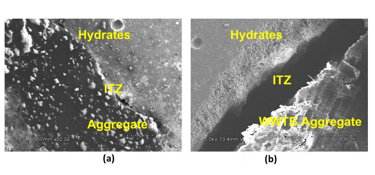
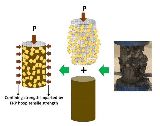
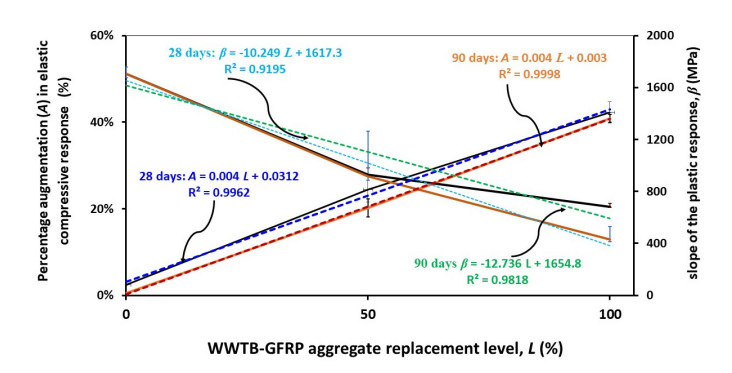
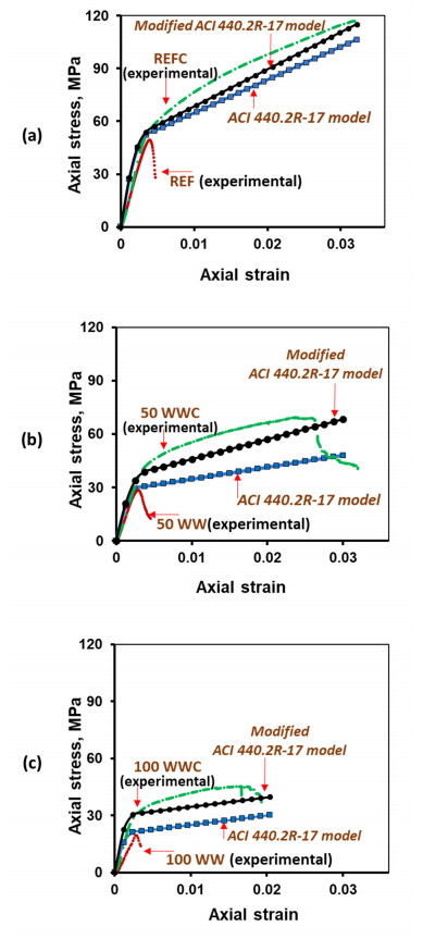
A major challenge in today's concrete construction is to lower its carbon footprint to the least possible level. This study provides insights on a new low-CO₂ alternative concrete whereby glass fiber-reinforced polymer (GFRP) materials from waste wind-turbine blades (WWTB)—termed as WWTB-GFRP—was utilized as: (ⅰ) replacement of Portland cement at 0%, 10%, 20%, and as (ⅱ) lightweight aggregate replacement for natural aggregates at 0%, 50%, and 100%. The resulting WWTB-GFRP concretes were used in concrete-filled fibre-reinforced polymer (FRP) tubes (CFFTs) whereby the latter serves as a stay-in-place formwork and external reinforcement. Pristine WWTB-GFRP materials (containing wood) and processed ones (by wood removal) were investigated. Results indicate that while both WWTB-GFRP powder and aggregates adversely affect the compression resistance (due to, respectively, the retarding effect of the powder and the slippery surface of the aggregates leading to reduced bonding with the bulk cementitious matrix), the confinement of WWTB-GFRP concrete with FRP tubes offers an innovative tool to restore the strength loss. In fact, valorizing WWTB-GFRP concrete in CFFTs allowed to increase the compressive resistance by more than 100%. Interestingly, under axial compression, FRP tube confinement shifted the stress–strain response from the conventional brittle response to a ductile one whereby the confinement affected the elastic and plastic responses differently. While FRP confinement increased in the elastic limit at higher WWTB-GFRP aggregate content, it resulted in lower slope of the plastic response at higher WWTB-GFRP aggregate content. An analytical assessment demonstrated that a WWTB-GFRP aggregate content of 55% will be optimum for enhancing both elastic and plastic responses. Building upon the ACI 440.2R-17 model for predicting the compressive response of confined concrete incorporating conventional aggregates, a modified model more sensitive to GFRP aggregates and with higher predictive ability was proposed. Research outcomes will contribute to recycling waste materials while endowing further sustainability to concrete.
Citation: Dmitry Baturkin, Ousmane A. Hisseine, Radhouane Masmoudi, Arezki Tagnit-Hamou, Slimane Metiche, Luc Massicotte. Compressive behavior of FRP-tube-confined concrete short columns using recycled FRP materials from wind turbine blades: Experimental investigation and analytical modelling[J]. Clean Technologies and Recycling, 2022, 2(3): 136-164. doi: 10.3934/ctr.2022008

Related Papers:

Abstract

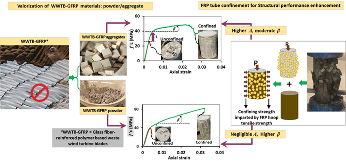
A major challenge in today's concrete construction is to lower its carbon footprint to the least possible level. This study provides insights on a new low-CO₂ alternative concrete whereby glass fiber-reinforced polymer (GFRP) materials from waste wind-turbine blades (WWTB)—termed as WWTB-GFRP—was utilized as: (ⅰ) replacement of Portland cement at 0%, 10%, 20%, and as (ⅱ) lightweight aggregate replacement for natural aggregates at 0%, 50%, and 100%. The resulting WWTB-GFRP concretes were used in concrete-filled fibre-reinforced polymer (FRP) tubes (CFFTs) whereby the latter serves as a stay-in-place formwork and external reinforcement. Pristine WWTB-GFRP materials (containing wood) and processed ones (by wood removal) were investigated. Results indicate that while both WWTB-GFRP powder and aggregates adversely affect the compression resistance (due to, respectively, the retarding effect of the powder and the slippery surface of the aggregates leading to reduced bonding with the bulk cementitious matrix), the confinement of WWTB-GFRP concrete with FRP tubes offers an innovative tool to restore the strength loss. In fact, valorizing WWTB-GFRP concrete in CFFTs allowed to increase the compressive resistance by more than 100%. Interestingly, under axial compression, FRP tube confinement shifted the stress–strain response from the conventional brittle response to a ductile one whereby the confinement affected the elastic and plastic responses differently. While FRP confinement increased in the elastic limit at higher WWTB-GFRP aggregate content, it resulted in lower slope of the plastic response at higher WWTB-GFRP aggregate content. An analytical assessment demonstrated that a WWTB-GFRP aggregate content of 55% will be optimum for enhancing both elastic and plastic responses. Building upon the ACI 440.2R-17 model for predicting the compressive response of confined concrete incorporating conventional aggregates, a modified model more sensitive to GFRP aggregates and with higher predictive ability was proposed. Research outcomes will contribute to recycling waste materials while endowing further sustainability to concrete.

References

[1]	GWEC, Global Wind Report Annual Market Update 2015. Global Wind Energy Council, 2015. Available form: https://www.gwec.net/wp-content/uploads/vip/GWEC-Global-Wind-2015-Report_April-2016_22_04.pdf.
[2]	Beauson J, Brøndsted P (2016) Wind turbine blades: An end of life perspective, In: Ostachowicz W, McGugan M, Schröder-Hinrichs JU, et al., MARE-WINT New Materials and Reliability in Offshore Wind Turbine Technology, Cham: Springer Nature, 421–432. https://doi.org/10.1007/978-3-319-39095-6_23
[3]	European Council, Conclusions on 2030 Climate and Energy Policy Framework. Council of the EU, 2014. Available form: http://www.consilium.europa.eu/en/press/press-releases/2014/10/pdf/European-Council-%2823-and-24-October-2014%29-Conclusions-on-2030-Climate-and-Energy-Policy-Framework/.
[4]	Canadian Renewable Energy Association, Wind Energy. Canadian Wind Energy Association, 2021. Available form: https://canwea.ca/wind-facts/why-wind-works/.
[5]	Fox T (2016) Recycling wind turbine blade composite material as aggregate in concrete [Master's thesis]. Iowa State University, United States.
[6]	Nagle AJ, Delaney EL, Bank LC, et al. (2020) A Comparative Life Cycle Assessment between landfilling and Co-Processing of waste from decommissioned Irish wind turbine blades. J Cleaner Prod 277: 123321. https://doi.org/10.1016/j.jclepro.2020.123321 doi: 10.1016/j.jclepro.2020.123321
[7]	D'Souza N, Gbegbaje-Das E, Shonfield P (2011) Life Cycle Assessment of Electricity Production from a Vestas V112 Turbine Wind Plant, Copenhagen: Vestas Wind Systems A/S.
[8]	Meira Castro AC, Carvalho JP, Ribeiro MCS, et al. (2014) An integrated recycling approach for GFRP pultrusion wastes: Recycling and reuse assessment into new composite materials using Fuzzy Boolean Nets. J Cleaner Prod 66: 420–430. https://doi.org/10.1016/j.jclepro.2013.10.030 doi: 10.1016/j.jclepro.2013.10.030
[9]	Correia JR, Almeida NM, Figueira JR (2011) Recycling of FRP composites: reusing fine GFRP waste in concrete mixtures. J Cleaner Prod 19: 1745–1753. https://doi.org/10.1016/j.jclepro.2011.05.018 doi: 10.1016/j.jclepro.2011.05.018
[10]	Asokan P, Osmani M, Price A (2010) Improvement of the mechanical properties of glass fibre reinforced plastic waste powder filled concrete. Constr Build Mater 24: 448–460. https://doi.org/10.1016/j.conbuildmat.2009.10.017 doi: 10.1016/j.conbuildmat.2009.10.017
[11]	Asokan P, Osmani M, Price ADF (2009) Assessing the recycling potential of glass fibre reinforced plastic waste in concrete and cement composites. J Cleaner Prod 17: 821–829. https://doi.org/10.1016/j.jclepro.2008.12.004 doi: 10.1016/j.jclepro.2008.12.004
[12]	Baturkin D, Hisseine OA, Masmoudi R, et al. (2021) Valorization of recycled FRP materials from wind turbine blades in concrete. Resour Conserv Recy 174: 105807. https://doi.org/10.1016/j.resconrec.2021.105807 doi: 10.1016/j.resconrec.2021.105807
[13]	Oliveira PS, Antunes MLP, da Cruz NC, et al. (2020) Use of waste collected from wind turbine blade production as an eco-friendly ingredient in mortars for civil construction. J Cleaner Prod 274: 122948. https://doi.org/10.1016/j.jclepro.2020.122948 doi: 10.1016/j.jclepro.2020.122948
[14]	Limbachiya MC (2004) Performance of recycled aggregate concrete, RILEM International Symposium on Environment-Conscious Materials and Systems for Sustainable Development, 127–136. https://doi.org/10.1617/2912143640.015 doi: 10.1617/2912143640.015
[15]	Hofmeister M (2012) Recycling turbine blade composites: Concrete aggregate and reinforcement, Wind Energy Science, Engineering and Policy Undergraduate Research Symposium Proceedings, 9/1–9/8.
[16]	Boumarafi A, Abouzied A, Masmoudi R (2015) Harsh environments effects on the axial behaviour of circular concrete-filled fibre reinforced-polymer (FRP) tubes. Compos Part B-Eng 83: 81–87. https://doi.org/10.1016/j.compositesb.2015.08.054 doi: 10.1016/j.compositesb.2015.08.054
[17]	Abouzied A, Masmoudi R (2017) Flexural behavior of rectangular FRP-tubes filled with reinforced concrete: Experimental and theoretical studies. Eng Struct 133: 59–73. https://doi.org/10.1016/j.engstruct.2016.12.010 doi: 10.1016/j.engstruct.2016.12.010
[18]	Mohamed H, Masmoudi R (2008) Compressive behavior of reinforced concrete-filled FRP tubes. American Concrete Institute (ACI) Special Publications, SP-257–06, ACI, Farmington Hills, Mich, 91–108.
[19]	Mohamed HM, Masmoudi R (2010) Axial load capacity of concrete-filled FRP tube columns: Experimental versus theoretical predictions. J Compos Constr 14: 231–243. https://doi.org/10.1061/(ASCE)CC.1943-5614.0000066 doi: 10.1061/(ASCE)CC.1943-5614.0000066
[20]	El-Zefzafy H, Mohamed HM, Masmoudi R (2013) Evaluation effects of the short-and long-term freeze-thaw exposure on the axial behavior of concrete-filled glass fiber-reinforced-polymer tubes. J Compos 2013: 340672. https://doi.org/10.1155/2013/340672 doi: 10.1155/2013/340672
[21]	ASTM C1157/C1157M-20a, Standard Performance Specification for Hydraulic Cement. ASTM International, 2021. Available from: https://www.astm.org/c1157_c1157m-20a.html.
[22]	ASTM C33/C33M-11, Standard Specification for Concrete Aggregates. ASTM International, 2011. Available from: https://www.astm.org/c0033_c0033m-11.html.
[23]	ACI 318-19, Building Code Requirements for Structural Concrete (ACI 318-19) and Commentary. ACI Committee, 2019. Available from: https://www.concrete.org/publications/internationalconcreteabstractsportal.aspx?m=details&ID=51716937.
[24]	ASTM C192/C192M-19, Standard Practice for Making and Curing Concrete Test Specimens in the Laboratory. ASTM International, 2016. Available from: https://www.astm.org/c0192_c0192m-19.html.
[25]	ASTM D4464-15, Standard Test Method for Particle Size Distribution of Catalytic Materials by Laser Light Scattering. ASTM International, 2020. Available from: https://www.astm.org/d4464-15r20.html.
[26]	ASTM D3039/D3039M-17, Standard Test Method for Tensile Properties of Polymer Matrix Composite Materials. ASTM International, 2017. Available from: https://www.astm.org/d3039_d3039m-17.html.
[27]	ASTM D695-15, Standard Test Method for Compressive Properties of Rigid Plastics. ASTM International, 2016. Available from: https://www.astm.org/d0695-15.html.
[28]	ASTM D2290-19a, Standard Test Method for Apparent Hoop Tensile Strength of Plastic or Reinforced Plastic Pipe. ASTM International, 2019. Available from: https://www.astm.org/Standards/D2290.htm.
[29]	ASTM C39/C39M-16, Standard Test Method for Compressive Strength of Cylindrical Concrete Specimens. ASTM International, 2016. Available from: https://www.astm.org/c0039_c0039m-16.html.
[30]	ACI PRC-440.2-17, Guide for the Design and Construction of Externally Bonded FRP Systems for Strengthening Concrete Structures. ACI Committee 440, 2017. Available from: https://www.concrete.org/store/productdetail.aspx?ItemID=440217&Language=English&Units=US_AND_METRIC.
[31]	Faella C, Lima C, Martinelli E, et al. (2016) Mechanical and durability performance of sustainable structural concretes: An experimental study. Cem Concr Compos 71: 85–96. https://doi.org/10.1016/j.cemconcomp.2016.05.009 doi: 10.1016/j.cemconcomp.2016.05.009
[32]	Lima C, Caggiano A, Faella C, et al. (2013) Physical properties and mechanical behaviour of concrete made with recycled aggregates and fly ash. Constr Build Mater 47: 547–559. https://doi.org/10.1016/j.conbuildmat.2013.04.051 doi: 10.1016/j.conbuildmat.2013.04.051
[33]	ACI 213R-14, Guide for Structural Lightweight-Aggregate Concrete. ACI Committee 213, 2014. Available from: https://www.concrete.org/store/productdetail.aspx?ItemID=21314&Language=English&Units=US_AND_METRIC.
[34]	Hisseine OA, Omran AF, Tagnit-Hamou A (2018) Influence of cellulose filaments on cement paste and concrete. J Mater Civil Eng 30: 04018109. https://doi.org/10.1061/(ASCE)MT.1943-5533.0002287 doi: 10.1061/(ASCE)MT.1943-5533.0002287
[35]	Jiang T, Teng JG (2007) Analysis-oriented stress–strain models for FRP-confined concrete. Eng Struct 29: 2968–2986. https://doi.org/10.1016/j.engstruct.2007.01.010 doi: 10.1016/j.engstruct.2007.01.010
[36]	Yang JQ, Feng P (2020) Analysis-oriented models for FRP-confined concrete: 3D interpretation and general methodology. Eng Struct 216: 110749. https://doi.org/10.1016/j.engstruct.2020.110749 doi: 10.1016/j.engstruct.2020.110749
[37]	Kwan AKH, Dong CX, Ho JCM (2015) Axial and lateral stress–strain model for FRP confined concrete. Eng Struct 99: 285–295. https://doi.org/10.1016/j.engstruct.2015.04.046 doi: 10.1016/j.engstruct.2015.04.046
[38]	Lam L, Teng JG (2003) Design-oriented stress–strain model for FRP-confined concrete. Constr Build Mater 17: 471–489. https://doi.org/10.1016/S0950-0618(03)00045-X doi: 10.1016/S0950-0618(03)00045-X

Reader Comments

Your name:*

Email:*
© 2022 the Author(s), licensee AIMS Press. This is an open access article distributed under the terms of the Creative Commons Attribution License (http://creativecommons.org/licenses/by/4.0)