Spatial twisted central configuration for Newtonian ($ 2N $+1)-body problem

Liang Ding; Jinrong Wang; Jinlong Wei; Liang Ding; Jinrong Wang; Jinlong Wei

doi:10.3934/cam.2024018

Communications in Analysis and Mechanics

2024, Volume 16, Issue 2: 388-415. doi: 10.3934/cam.2024018

Previous Article Next Article

Research article

Spatial twisted central configuration for Newtonian ($ 2N $+1)-body problem

1.
Department of Mathematics, Guizhou University, Guiyang, 550025, P.R. China
2.
School of Data Science and Information Engineering, Guizhou Minzu University, Guiyang, 550025, P.R. China
3.
School of Statistics and Mathematics, Zhongnan University of Economics and Law, Wuhan, 430073, P.R. China

Received: 04 November 2023 Revised: 11 March 2024 Accepted: 10 April 2024 Published: 20 May 2024
70F10, 70F15

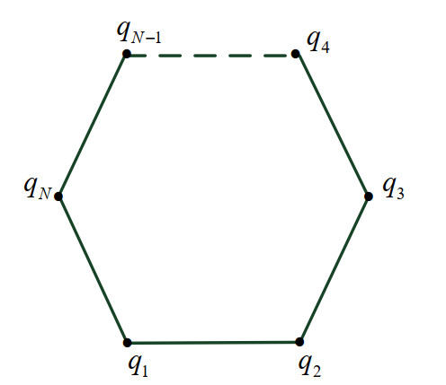
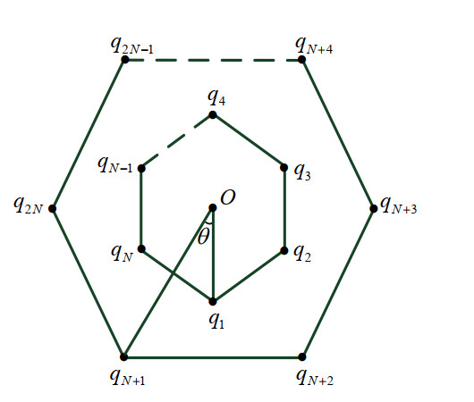
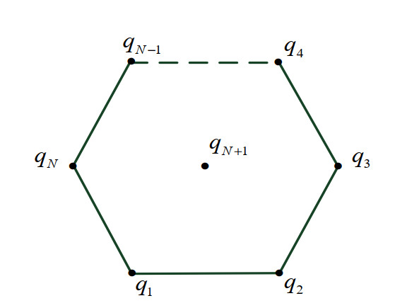
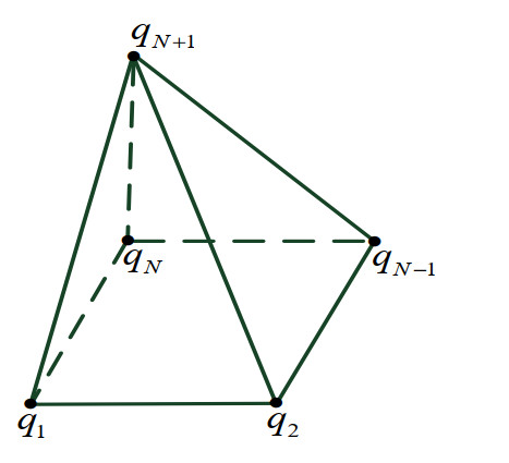
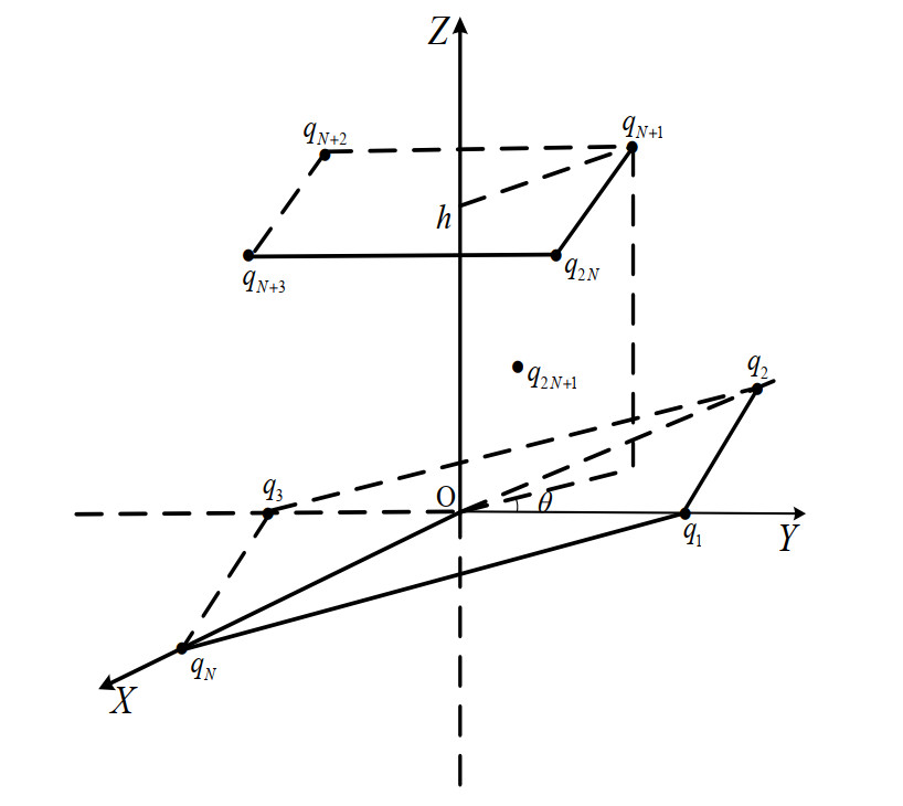
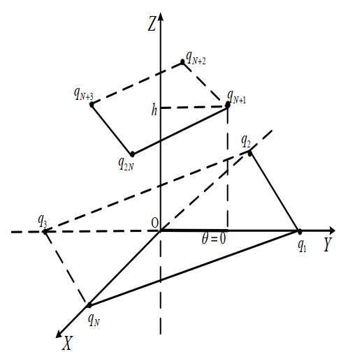
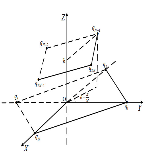
For a spatial twisted central configuration of the Newtonian ($ 2N $+1)-body problem where $ 2N $ masses are at the vertices of two paralleled regular $ N $-polygons with distance $ h > 0 $, and the twist angle between the two regular $ N $-polygons is $ 0\leq\theta < 2\pi $, we study the sufficient and necessary conditions for the existence of the spatial twisted central configuration. Additionally, we obtain the uniqueness of the spatial twisted central configuration.
- Newtonian ($ 2N $+1)-body problem,
- spatial central configuration,
- regular $ N $-polygons,
- twist angle
Citation: Liang Ding, Jinrong Wang, Jinlong Wei. Spatial twisted central configuration for Newtonian ($ 2N $+1)-body problem[J]. Communications in Analysis and Mechanics, 2024, 16(2): 388-415. doi: 10.3934/cam.2024018

Related Papers:

Abstract

For a spatial twisted central configuration of the Newtonian ($ 2N $+1)-body problem where $ 2N $ masses are at the vertices of two paralleled regular $ N $-polygons with distance $ h > 0 $, and the twist angle between the two regular $ N $-polygons is $ 0\leq\theta < 2\pi $, we study the sufficient and necessary conditions for the existence of the spatial twisted central configuration. Additionally, we obtain the uniqueness of the spatial twisted central configuration.

References

[1]	A. Wintner, The analytical foundations of celestial mechanics, Princeton University Press, New Jersey, 1941.
[2]	L. Euler, De moto rectilineo trium corporum se mutuo attrahentium, Novi. Comm. Acad. Sci. Imp. Petrop., 11 (1767), 144–151.
[3]	J. Lagrange, Essai sur le problème des trois crops, Œuvres, 6 (1772), 229–324.
[4]	L. Perko, E. Walter, Regular polygon solutions of the $N$-body problem, Proc. Amer. Math. Soc., 94 (1985), 301–309. https://doi.org/10.1090/S0002-9939-1985-0784183-1 doi: 10.1090/S0002-9939-1985-0784183-1
[5]	M. Corbera, C. Valls, On centered co-circular central configurations of the $n$-body problem, J. Dyn. Differ. Equ., 31 (2019), 2053–2060. https://doi.org/10.1007/s10884-018-9699-2 doi: 10.1007/s10884-018-9699-2
[6]	W. Li, Z. Q. Wang, The relationships between regular polygon central configurations and masses for Newtonian $N$-body problems, Phys. Lett. A, 377 (2013), 1875–1880. https://doi.org/10.1016/j.physleta.2013.05.044 doi: 10.1016/j.physleta.2013.05.044
[7]	J. Llibre, R. Moeckel, C. Simó, Central configurations, periodic orbits, and Hamiltonian systems, Birkhäuser, New York, 2015. https://doi.org/10.1007/978-3-0348-0933-7
[8]	D. G. Saari, On the role and the properties of $n$ body central configurations, Celest. Mech., 21 (1980), 9–20. https://doi.org/10.1007/bf01230241 doi: 10.1007/bf01230241
[9]	S. Q. Zhang, Q. Zhou, Periodic solutions for planar $2N$-body problems, Proc. Amer. Math. Soc., 131 (2003), 2161–2170. https://doi.org/10.1090/S0002-9939-02-06795-3 doi: 10.1090/S0002-9939-02-06795-3
[10]	R. Moeckel, C. Simó, Bifurcation of spatial central configurations from planar ones, SIAM. J. Math. Anal., 26 (1995), 978–998. https://doi.org/10.1137/S0036141093248414 doi: 10.1137/S0036141093248414
[11]	E. Barrabés, J. M. Cors, On central configurations of the $\kappa n$-body problem, J. Math. Anal. Appl., 476 (2) (2019), 720–736. https://doi.org/10.1016/j.jmaa.2019.04.010
[12]	M. Corbera, J. Delgado, J. Llibre, On the existence of central configurations of $p$ nested $n$-gons, Qual. Theory Dyn. Syst., 8 (2009), 255–265. https://doi.org/10.1007/s12346-010-0004-y doi: 10.1007/s12346-010-0004-y
[13]	F. Zhao, J. Chen, Central configurations for $(pN+gN)$-body problems, Celest. Mech. Dyn. Astr., 121 (1) (2015), 101–106. https://10.1007/s10569-014-9593-0
[14]	J. Lei, M. Santoprete, Rosette central configurations, degenerate central configurations and bifurcations, Celest. Mech. Dyn. Astr., 94 (2006), 271–287. https://doi.org/10.1007/s10569-005-5534-2 doi: 10.1007/s10569-005-5534-2
[15]	J. Llibre, L. F. Mello, Triple and quadruple nested central configurations for the planar $n$-body problem, Physica D, 238 (2009), 563–571. https://doi.org/10.1016/j.physd.2008.12.014 doi: 10.1016/j.physd.2008.12.014
[16]	M. Marchesin, A family of three nested regular polygon central configurations, Astrophys. Space Sci., 364 (2019), 1–12. https://doi.org/10.1007/s10509-019-3648-3 doi: 10.1007/s10509-019-3648-3
[17]	A. Siluszyk, On a class of central configurations in the planar $3n$-body problem, Math. Comput. Sci., 11 (2017), 457–467. http://dx.doi.org/10.1007/s11786-017-0309-1 doi: 10.1007/s11786-017-0309-1
[18]	Z. Q. Wang, F. Y. Li, A note on the two nested regular polygonal central configurations, Proc. Amer. Math. Soc., 143 (2015), 4817–4822. https://doi.org/10.1090/S0002-9939-2015-12618-4 doi: 10.1090/S0002-9939-2015-12618-4
[19]	Z. F. Xie, G. Bhusal, H. Tahir, Central configurations in the planar 6-body problem forming two equilateral triangles, J. Geom. Phys., 153 (2020), 1–11. https://doi.org/10.1016/j.geomphys.2020.103645 doi: 10.1016/j.geomphys.2020.103645
[20]	S. Q. Zhang, C. R. Zhu, Central configurations consist of two layer twisted regular polygons, Sci. China Ser. A, 45 (2002), 1428–1438. https://doi.org/10.1007/BF02880037 doi: 10.1007/BF02880037
[21]	X. Yu, S. Q. Zhang, Central configurations formed by two twisted regular polygons, J. Math. Anal. Appl., 425 (2015), 372–380. https://doi.org/10.1016/j.jmaa.2014.12.023 doi: 10.1016/j.jmaa.2014.12.023
[22]	J. Chen, J. B. Luo, Solutions of regular polygon with an inner particle for Newtonian $N$+1-body problem, J. Differ. Equ., 265 (2018), 1248–1258. https://doi.org/10.1016/j.jde.2018.04.004 doi: 10.1016/j.jde.2018.04.004
[23]	T. Ouyang, Z. F. Xie, S. Q. Zhang, Pyramidal central configurations and perverse solutions, Electron. J. Differ. Equ., 1 (2004), 1–9.
[24]	X. Yu, S. Q. Zhang, Twisted angles for central configurations formed by two twisted regular polygons, J. Differ. Equ., 253 (2012), 2106–2122. https://doi.org/10.1016/j.jde.2012.06.017 doi: 10.1016/j.jde.2012.06.017
[25]	M. Marcus, H. Minc, A survey of matrix theory and matrix inequalities, Allyn & Bacon, Boston, 1964.
[26]	L. Ding, J. L. Wei, S. Q. Zhang, The central configuration of the planar ($N$+1)-body problem with a regular $N$-polygon for homogeneous force laws, Astrophys. Space Sci., 367 (2022), 1–9. https://doi.org/10.1007/s10509-022-04095-w doi: 10.1007/s10509-022-04095-w

Reader Comments

Your name:*

Email:*
© 2024 the Author(s), licensee AIMS Press. This is an open access article distributed under the terms of the Creative Commons Attribution License (http://creativecommons.org/licenses/by/4.0)