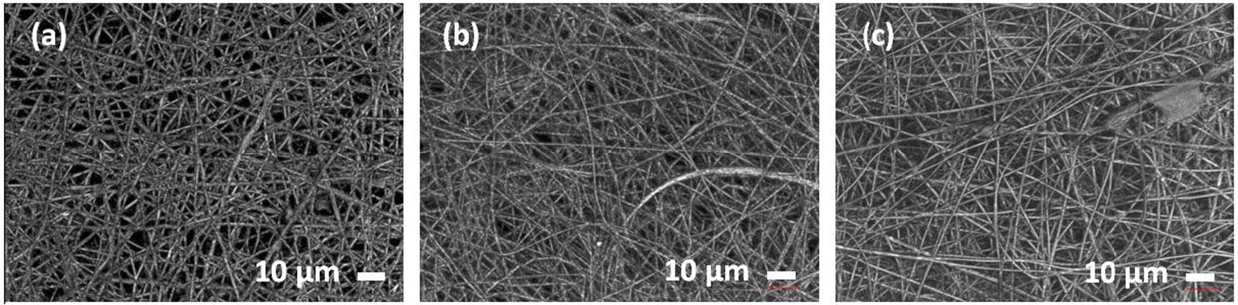
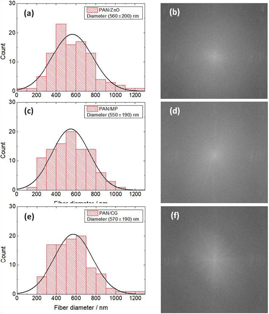
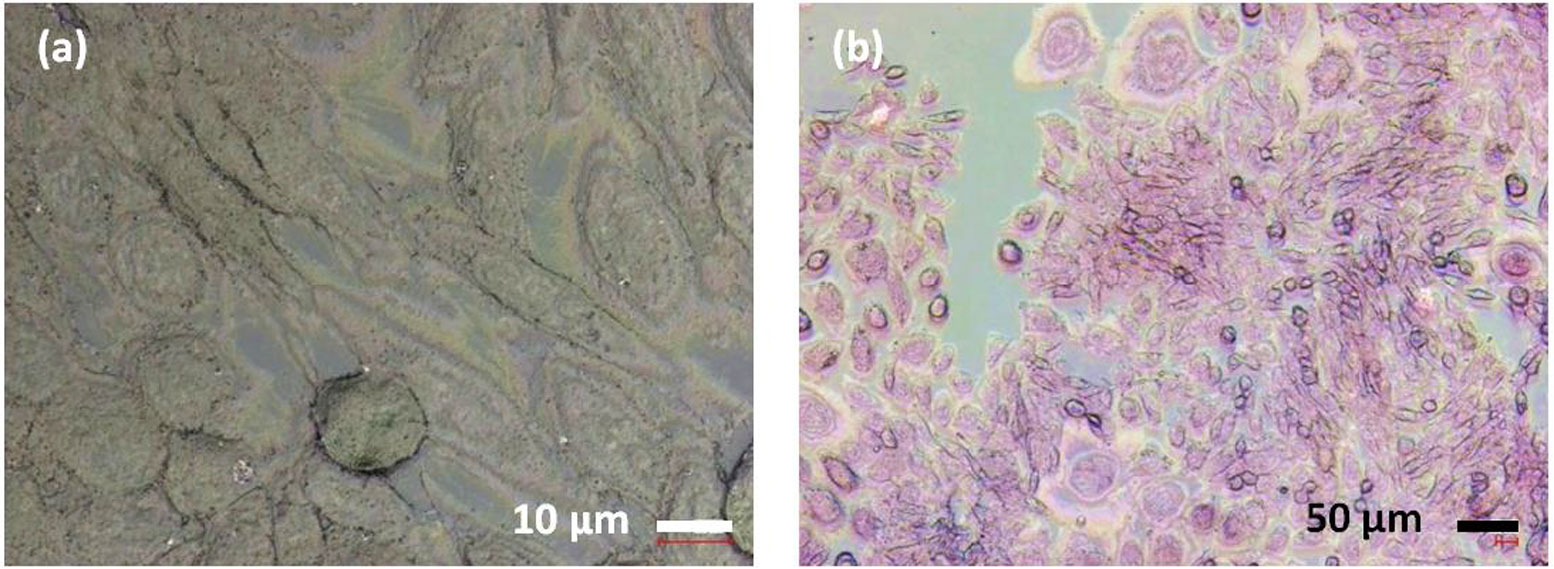
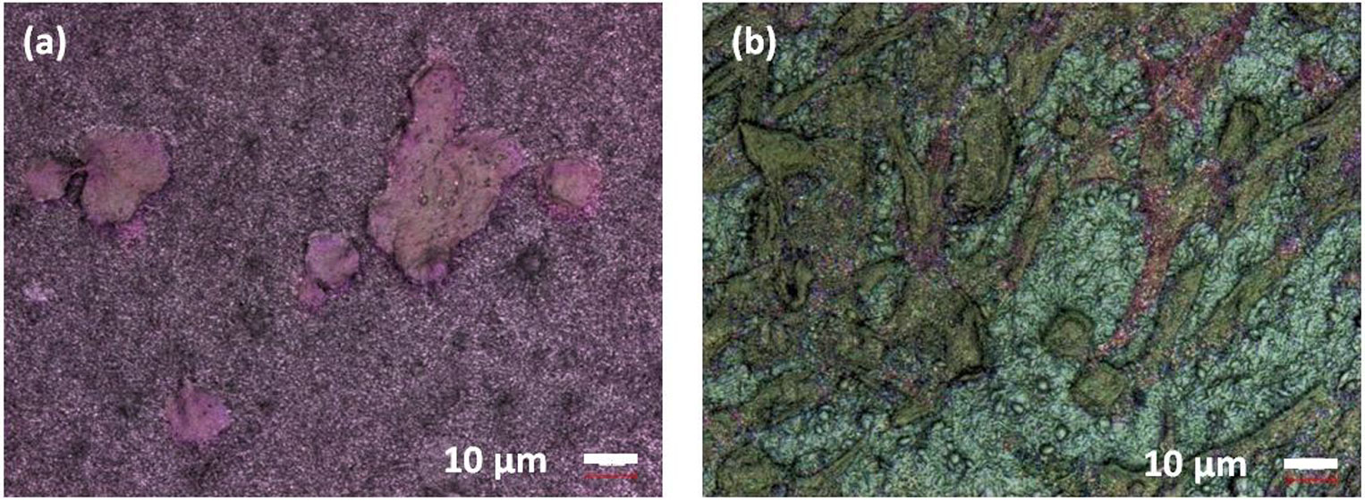
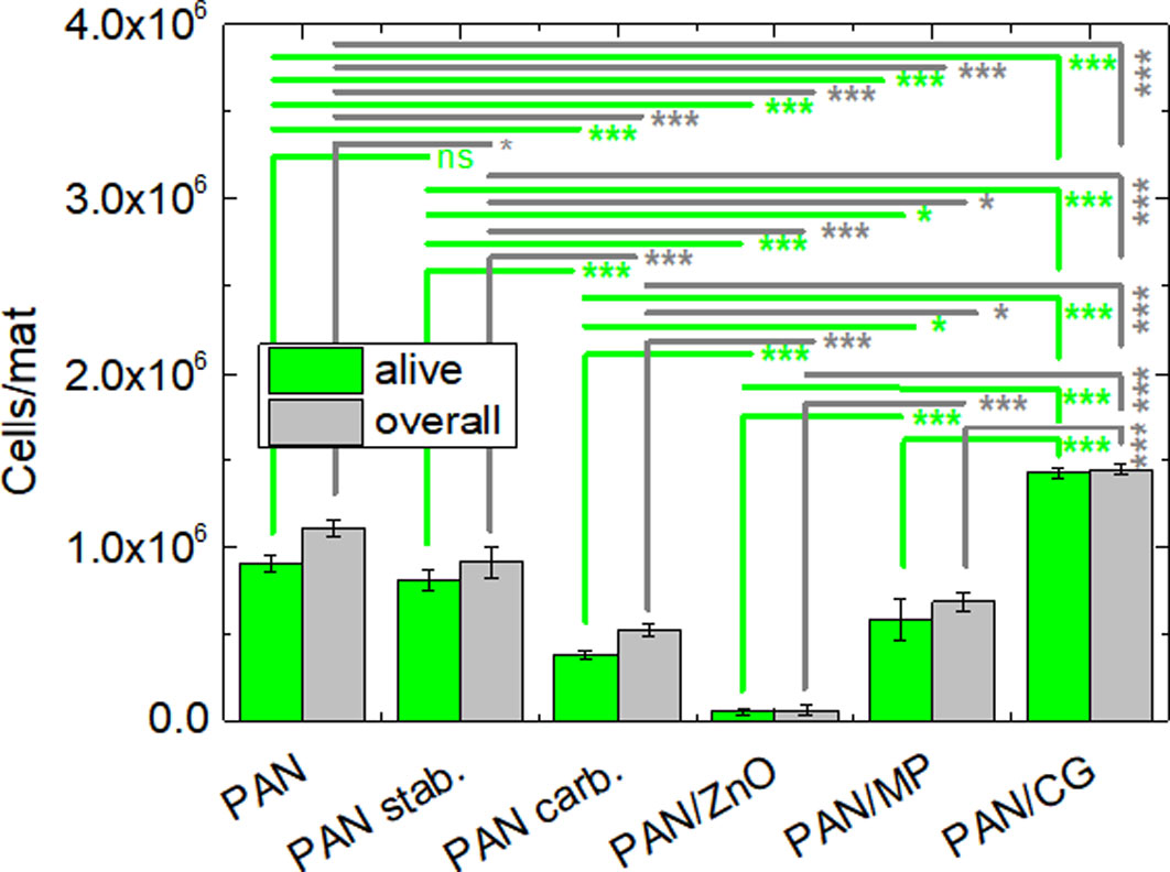
Nanofiber mats can be produced by electrospinning from diverse polymers and polymer blends as well as with embedded ceramics, metals, etc. The large surface-to-volume ratio makes such nanofiber mats a well-suited substrate for tissue engineering and other cell growth experiments. Cell growth, however, is not only influenced by the substrate morphology, but also by the sterilization process applied before the experiment as well as by the chemical composition of the fibers. A former study showed that cell growth and adhesion are supported by polyacrylonitrile/gelatin nanofiber mats, while both factors are strongly reduced on pure polyacrylonitrile (PAN) nanofibers. Here we report on the influence of different PAN blends on cell growth and adhesion. Our study shows that adding ZnO to the PAN spinning solution impedes cell growth, while addition of maltodextrin/pea protein or casein/gelatin supports cell growth and adhesion.
Citation: Daria Wehlage, Hannah Blattner, Al Mamun, Ines Kutzli, Elise Diestelhorst, Anke Rattenholl, Frank Gudermann, Dirk Lütkemeyer, Andrea Ehrmann. Cell growth on electrospun nanofiber mats from polyacrylonitrile (PAN) blends[J]. AIMS Bioengineering, 2020, 7(1): 43-54. doi: 10.3934/bioeng.2020004
Nanofiber mats can be produced by electrospinning from diverse polymers and polymer blends as well as with embedded ceramics, metals, etc. The large surface-to-volume ratio makes such nanofiber mats a well-suited substrate for tissue engineering and other cell growth experiments. Cell growth, however, is not only influenced by the substrate morphology, but also by the sterilization process applied before the experiment as well as by the chemical composition of the fibers. A former study showed that cell growth and adhesion are supported by polyacrylonitrile/gelatin nanofiber mats, while both factors are strongly reduced on pure polyacrylonitrile (PAN) nanofibers. Here we report on the influence of different PAN blends on cell growth and adhesion. Our study shows that adding ZnO to the PAN spinning solution impedes cell growth, while addition of maltodextrin/pea protein or casein/gelatin supports cell growth and adhesion.

| [1] |
Dizge N, Shaulsky E, Karanikola V (2019) Electrospun cellulose nanofibers for superhydrophobic and oleophobic membranes. J Membr Sci 590: 117271. doi: 10.1016/j.memsci.2019.117271

|
| [2] |
Pavlova ER, Bagrov DV, Monakhova KZ, et al. (2019) Tuning the properties of electrospun polylactide mats by ethanol treatment. Mater Des 181: 108061. doi: 10.1016/j.matdes.2019.108061
|
| [3] | Wang JN, Zhao WW, Wang B, et al. (2017) Multilevel-layer-structured polyamide 6/poly(trimethylene terephthalate) nanofibrous membranes for low-pressure air filtration. J Appl Pol Sci 134: 44716. |
| [4] |
Cooper A, Oldinski R, Ma H Y, et al. (2013) Chitosan-based nanofibrous membranes for antibacterial filter applications. Carbohyd Polym 92: 254-259. doi: 10.1016/j.carbpol.2012.08.114
|
| [5] |
Banner J, Dautzenberg M, Feldhans T, et al. (2018) Water resistance and morphology of electrospun gelatine blended with citric acid and coconut oil. Tekstilec 61: 129-135. doi: 10.14502/Tekstilec2018.61.129-135
|
| [6] |
Grimmelsmann N, Homburg SV, Ehrmann A (2017) Electrospinning chitosan blends for nonwovens with morphologies between nanofiber mat and membrane. IOP Conf Series Mater Sci Eng 213: 012007. doi: 10.1088/1757-899X/213/1/012007
|
| [7] |
Wortmann M, Freese N, Sabantina L, et al. (2019) New polymers for needleless electrospinning from low-toxic solvents. Nanomater 9: 52. doi: 10.3390/nano9010052
|
| [8] |
Krasonu I, Tarassova E, Malmberg S, et al. (2019) Preparation of fibrous electrospun membranes with activated carbon filler. IOP Conf Series Mater Sci Eng 500: 012022. doi: 10.1088/1757-899X/500/1/012022
|
| [9] |
Plamus T, Savest N, Viirsalu M, et al. (2018) The effect of ionic liquids on the mechanical properties of electrospun polyacrylonitrile membranes. Polym Test 71: 335-343. doi: 10.1016/j.polymertesting.2018.09.003
|
| [10] |
Sabantina L, Mirasol JR, Cordero T, et al. (2018) Investigation of needleless electrospun PAN nanofiber mats. AIP Conf Proc 1952: 020085. doi: 10.1063/1.5032047
|
| [11] |
Wang JH, Cai C, Zhang ZJ, et al. (2020) Electrospun metal-organic frameworks with polyacrylonitrile as precursors to hierarchical porous carbon and composite nanofibers for adsorption and catalysis. Chemosphere 239: 124833. doi: 10.1016/j.chemosphere.2019.124833
|
| [12] |
de Oliveira JB, Guerrini LM, dos Santos Conejo L, et al. (2019) Viscoelastic evaluation of epoxy nanocomposite based on carbon nanofiber obtained from electrospinning processing. Polym Bull 76: 6063-6076. doi: 10.1007/s00289-019-02707-0
|
| [13] |
Trabelsi M, Mamun A, Klöcker M, et al. (2019) Increased mechanical properties of carbon nanofiber mats for possible medical applications. Fibers 7: 98. doi: 10.3390/fib7110098
|
| [14] |
Wang L, Zhang C, Gao F, et al. (2016) Needleless electrospinning for scaled-up production of ultrafine chitosan hybrid nanofibers used for air filtration. RSC Adv 6: 105988-105995. doi: 10.1039/C6RA24557A
|
| [15] |
Roche R, Yalcinkaya F (2018) Incorporation of PVDF nanofibre multilayers into functional structure for filtration applications. Nanomater 8: 771. doi: 10.3390/nano8100771
|
| [16] |
Lv D, Wang RX, Tang GS, et al. (2019) Ecofriendly electrospun membranes loaded with visible-light-responding nanoparticles for multifunctional usages: highly efficient air filtration, dye scavenging, and bactericidal activity. ACS Appl Mater Interfaces 11: 12880-12889. doi: 10.1021/acsami.9b01508
|
| [17] |
Fu QS, Lin G, Chen XD, et al. (2018) Mechanically reinforced PVdF/PMMA/SiO2 composite membrane and its electrochemical properties as a separator in lithium-ion batteries. Energy Technol 6: 144-152. doi: 10.1002/ente.201700347
|
| [18] |
Mamun A, Trabelsi M, Klöcker M, et al. (2019) Electrospun nanofiber mats with embedded non-sintered TiO2 for dye sensitized solar cells (DSSCs). Fibers 7: 60. doi: 10.3390/fib7070060
|
| [19] |
Xue YY, Guo X, Zhou HF, et al. (2019) Influence of beads-on-string on Na-Ion storage behavior in electrospun carbon nanofibers. Carbon 154: 219-229. doi: 10.1016/j.carbon.2019.08.003
|
| [20] |
Mamun A (2019) Review of possible applications of nanofibrous mats for wound dressings. Tekstilec 62: 89-100. doi: 10.14502/Tekstilec2019.62.89-100
|
| [21] |
Gao ST, Tang GS, Hua DW, et al. (2019) Stimuli-responsive bio-based polymeric systems and their applications. J Mater Chem B 7: 709-729. doi: 10.1039/C8TB02491J
|
| [22] |
Aljawish A, Muniglia L, Chevalot I (2016) Growth of human mesenchymal stem cells (MSCs) on films of enzymatically modified chitosan. Biotechnol Prog 32: 491-500. doi: 10.1002/btpr.2216
|
| [23] |
Muzzarelli RAA, EI Mehtedi M, Bottegoni C, et al. (2015) Genipin-crosslinked chitosan gels and scaffolds for tissue engineering and regeneration of cartilage and bone. Mar Drugs 13: 7314-7338. doi: 10.3390/md13127068
|
| [24] |
Klinkhammer K, Seiler N, Grafahrend D, et al. (2009) Deposition of electrospun fibers on reactive substrates for in vitro investigations. Tissue Eng Part C 15: 77-85. doi: 10.1089/ten.tec.2008.0324
|
| [25] |
Yoshida H, Klinkhammer K, Matsusaki M, et al. (2009) Disulfide-crosslinked electrospun poly(γ-glutamic acid) nonwovens as reduction-responsive scaffolds. Macromol Biosci 9: 568-574. doi: 10.1002/mabi.200800334
|
| [26] | Chatel A (2019) A brief history of adherent cell culture: where we come from and where we should go. BioProcess Int 17: 44-49. |
| [27] | Whitford WG, Hardy JC, Cadwell JJS (2014) Single-use, continuous processing of primary stem cells. BioProcess Int 12: 26-32. |
| [28] | Simon M (2015) Bioreactor design for adherent cell culture. The bolt-on bioreactor project, part 1: volumetric productivity. BioProcess Int 13: 28-33. |
| [29] |
Allan SJ, De Bank PA, Ellis MJ (2019) Bioprocess design considerations for cultured meat production with a focus on the expansion bioreactor. Front Sus Food Syst 3: 44. doi: 10.3389/fsufs.2019.00044
|
| [30] | GE Healthcare Life Sciences (2013) Microcarrier Cell Culture, Principles and Methods.Available from: http://www.gelifesciences.co.kr/wp-content/uploads/2016/07/023.8_Microcarrier-Cell-Culture.pdf. |
| [31] |
Lennaertz A, Knowles S, Drugmand JC, et al. (2013) Viral vector production in the integrity iCELLis single-use fixed-bed bioreactor, from bench-scale to industrial scale. BMC Proc 7: P59. doi: 10.1186/1753-6561-7-S6-P59
|
| [32] | Dohogne Y, Collignon F, Drugmand JC, et al. (2019) Scale-X bioreactor for viral vector production. Proof of concept for scalable HEK293 cell growth and adenovirus production, Univercell Application note.Available from: https://www.univercells.com/app/uploads/2019/05/scale-X%E2%84%A2-bioreactor-for-viral-production-Adeno_SFM.pdf. |
| [33] |
Drugmand JC, Aghatos S, Schneider YJ, et al. (2007) Growth of mammalian and lepidopteram cells on BioNOC® II disks, a novel macroporous microcarrier. Cell Technology for Cell Products Heidelberg: Springer, 781-784. doi: 10.1007/978-1-4020-5476-1_143
|
| [34] |
Wehlage D, Blatter H, Sabantina L, et al. (2019) Sterilization of PAN/gelatin nanofibrous mats for cell growth. Tekstilec 62: 78-88. doi: 10.14502/Tekstilec2019.62.78-88
|
| [35] |
Ghasemi A, Imani R, Yousefzadeh M, et al. (2019) Studying the potential application of electrospun polyethylene terephthalate/graphene oxide nanofibers as electroconductive cardiac patc. Macromol Mater Eng 304: 1900187. doi: 10.1002/mame.201900187
|
| [36] |
Nekouian S, Sojoodi M, Nadri S (2019) Fabrication of conductive fibrous scaffold for photoreceptor differentiation of mesenchymal stem cell. J Cell Physiol 234: 15800-15808. doi: 10.1002/jcp.28238
|
| [37] |
Rahmani A, Nadri S, Kazemi HS, et al. (2019) Conductive electrospun scaffolds with electrical stimulation for neural differentiation of conjunctiva mesenchymal stem cells. Artif Organs 43: 780-790. doi: 10.1111/aor.13425
|
| [38] | Kutzli I, Beljo D, Gibis M, et al. (2019) Effect of maltodextrin dextrose equivalent on electrospinnability and glycation reaction of blends with pea protein isolate. Food Biophysics . |
| [39] |
Diestelhorst E, Mance F, Mamun A, et al. (2020) Chemical and morphological modification of PAN nanofiber mats by addition of casein after electrospinning, stabilization and carbonization. Tekstilec 63: 38-49. doi: 10.14502/Tekstilec2020.63.38-49
|
| [40] |
Möller J, Korte K, Pörtner R, et al. (2018) Model-based identification of cell-cycle-dependent metabolism and putative autocrine effects in antibody producing CHO cell culture. Biotechnol Bioeng 115: 2996-3008. doi: 10.1002/bit.26828
|
| [41] |
Wippermann A, Rupp O, Brinkrolf K, et al. (2015) The DNA methylation landscape of Chinese hamster ovary (CHO) DP-12 cells. J Biotechnol 199: 38-46. doi: 10.1016/j.jbiotec.2015.02.014
|
| [42] |
Haredy AM, Nishizawa A, Honda K, et al. (2013) Improved antibody production in Chinese hamster ovary cells by ATF4 overexpression. Cytotechnology 65: 993-1002. doi: 10.1007/s10616-013-9631-x
|
| [43] |
Bazrafshan Z, Stylios GK (2018) Custom-built electrostatics and supplementary bonding in the design of reinforced Collagen-g-P (methyl methacrylate-co-ethyl acrylate)/nylon 66 core-shell fibers. J Mech Behav Biomed Mater 87: 19-29. doi: 10.1016/j.jmbbm.2018.07.002
|
| [44] |
Storck JL, Grothe T, Mamun A, et al. (2020) Orientation of electrospun magnetic nanofibers near conductive areas. Materials 13: 47. doi: 10.3390/ma13010047
|
| [45] |
Richter KN, Revelo NH, Seitz KJ, et al. (2018) Glyoxal as an alternative fixative to formaldehyde in immunostaining and super-resolution microscopy. EMBO J 37: 139-159. doi: 10.15252/embj.201695709
|
| [46] |
Huang LC, Lin W, Yagami M, et al. (2010) Validation of cell density and viability assays using Cedex automated cell counter. Biologicals 38: 393-400. doi: 10.1016/j.biologicals.2010.01.009
|
| [47] |
Sabantina L, Rodríguez-Cano MA, Klöcker M, et al. (2018) Fixing PAN nanofiber mats during stabilization for carbonization and creating novel metal/carbon composites. Polymers 10: 735. doi: 10.3390/polym10070735
|
| [48] |
Baek M, Kim MK, Cho HJ, et al. (2011) Factors influencing the cytotoxicity of zinc oxide nanoparticles: particle size and surface charge. J Phys Conf Ser 304: 012044. doi: 10.1088/1742-6596/304/1/012044
|
| [49] |
Sing S (2019) Zinc oxide nanoparticles impacts: cytotoxicity, genotoxicity, development toxicity, and neurotoxicity. Toxicol Mech Methods 29: 300-311. doi: 10.1080/15376516.2018.1553221
|
| [50] |
Kuebodeaux RE, Bernazzani P, Nguyen TTM (2018) Cytotoxic and membrane cholesterol effects of ultraviolet irradiation and zinc oxide nanoparticles on Chinese hamster ovary cells. Molecules 23: 2979. doi: 10.3390/molecules23112979
|
| [51] |
Zukiene R, Snitka V (2015) Zinc oxide nanoparticle and bovine serum albumin interaction andnanoparticles influence on cytotoxicity in vitro. Colloids Surf B 135: 316-323. doi: 10.1016/j.colsurfb.2015.07.054
|
Figures(8) / Tables(1)

Daria Wehlage, Hannah Blattner, Al Mamun, Ines Kutzli, Elise Diestelhorst, Anke Rattenholl, Frank Gudermann, Dirk Lütkemeyer, Andrea Ehrmann. Cell growth on electrospun nanofiber mats from polyacrylonitrile (PAN) blends[J]. AIMS Bioengineering, 2020, 7(1): 43-54. doi: 10.3934/bioeng.2020004


 DownLoad: