Semi-supervised multiscale dual-encoding method for faulty traffic data detection

Yongcan Huang; Jidong J. Yang; Yongcan Huang; Jidong J. Yang

doi:10.3934/aci.2022006

Applied Computing and Intelligence

2022, Volume 2, Issue 2: 99-114. doi: 10.3934/aci.2022006

Previous Article Next Article

Research article

Semi-supervised multiscale dual-encoding method for faulty traffic data detection

Yongcan Huang ,
Jidong J. Yang ^,

Smart Mobility and Infrastructure Laboratory, College of Engineering, University of Georgia, Athens GA, USA

Received: 11 July 2022 Revised: 19 August 2022 Accepted: 12 September 2022 Published: 16 September 2022

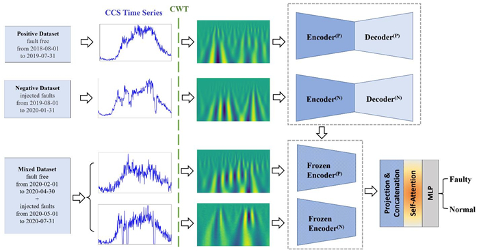
Inspired by the recent success of deep learning in multiscale information encoding, we introduce a variational autoencoder (VAE) based semi-supervised method for detection of faulty traffic data, which is cast as a classification problem. Continuous wavelet transform (CWT) is applied to the time series of traffic volume data to obtain rich features embodied in time-frequency representation, followed by a twin of VAE models to separately encode normal data and faulty data. The resulting multiscale dual encodings are concatenated and fed to an attention-based classifier, consisting of a self-attention module and a multilayer perceptron. For comparison, the proposed architecture is evaluated against five different encoding schemes, including (1) VAE with only normal data encoding, (2) VAE with only faulty data encoding, (3) VAE with both normal and faulty data encodings, but without attention module in the classifier, (4) siamese encoding, and (5) cross-vision transformer (CViT) encoding. The first four encoding schemes adopt the same convolutional neural network (CNN) architecture while the fifth encoding scheme follows the transformer architecture of CViT. Our experiments show that the proposed architecture with the dual encoding scheme, coupled with attention module, outperforms other encoding schemes and results in classification accuracy of 96.4%, precision of 95.5%, and recall of 97.7%.
- faulty data detection,
- continuous wavelet transform,
- variational autoencoder,
- self-attention,
- semi-supervised learning
Citation: Yongcan Huang, Jidong J. Yang. Semi-supervised multiscale dual-encoding method for faulty traffic data detection[J]. Applied Computing and Intelligence, 2022, 2(2): 99-114. doi: 10.3934/aci.2022006

Related Papers:

Abstract

Inspired by the recent success of deep learning in multiscale information encoding, we introduce a variational autoencoder (VAE) based semi-supervised method for detection of faulty traffic data, which is cast as a classification problem. Continuous wavelet transform (CWT) is applied to the time series of traffic volume data to obtain rich features embodied in time-frequency representation, followed by a twin of VAE models to separately encode normal data and faulty data. The resulting multiscale dual encodings are concatenated and fed to an attention-based classifier, consisting of a self-attention module and a multilayer perceptron. For comparison, the proposed architecture is evaluated against five different encoding schemes, including (1) VAE with only normal data encoding, (2) VAE with only faulty data encoding, (3) VAE with both normal and faulty data encodings, but without attention module in the classifier, (4) siamese encoding, and (5) cross-vision transformer (CViT) encoding. The first four encoding schemes adopt the same convolutional neural network (CNN) architecture while the fifth encoding scheme follows the transformer architecture of CViT. Our experiments show that the proposed architecture with the dual encoding scheme, coupled with attention module, outperforms other encoding schemes and results in classification accuracy of 96.4%, precision of 95.5%, and recall of 97.7%.

References

[1]	Transportation Research Board, Advancing Highway Traffic Monitoring Through Strategic Research, Transportation Research Circular E-C227, 2017.
[2]	S. Turner, Defining and measuring traffic data quality: White paper on recommended approaches, Transport. Res. Rec., 1870 (2004), 62–69. https://doi.org/10.3141/1870-08 doi: 10.3141/1870-08
[3]	C. L. Wen, F. Y. Lv, Z. J. Bao, M. Q. Liu, A review of data driven-based incipient fault diagnosis, Acta Automatica Sinica, 42 (2016), 1285–1299.
[4]	W. Bounoua, A. Bakdi, Fault detection and diagnosis of nonlinear dynamical processes through correlation dimension and fractal analysis based dynamic kernel PCA, Chem. Eng. Sci., 229 (2021), 116099. https://doi.org/10.1016/j.ces.2020.116099 doi: 10.1016/j.ces.2020.116099
[5]	R. Rubini, U. Meneghetti, Application of the envelope and wavelet transform analyses for the diagnosis of incipient faults in ball bearings, Mech. Syst. Signal Process., 15 (2001), 287–302. https://doi.org/10.1006/mssp.2000.1330 doi: 10.1006/mssp.2000.1330
[6]	E. Aker, M. L. Othman, V. Veerasamy, I. B. Aris, N. I. A. Wahab, H. Hizam, Fault detection and classification of shunt compensated transmission line using discrete wavelet transform and naive bayes classifier, Energies, 13 (2020), 243. https://doi.org/10.3390/en13010243 doi: 10.3390/en13010243
[7]	M. Rhif, A. ben Abbes, I. R. Farah, B. Martinez, Y. Sang, Wavelet transform application for/in non-stationary time-series analysis: a review. Applied Sciences, 9 (2019), 1345. https://doi.org/10.3390/app9071345 doi: 10.3390/app9071345
[8]	D. Jiang, C. Yao, Z. Xu, W. Qin, Multi‐scale anomaly detection for high‐speed network traffic, T. Emerg. Telecommun. T., 26 (2015), 308–317. https://doi.org/10.1002/ett.2619 doi: 10.1002/ett.2619
[9]	E. Ayaz, A. Öztürk, S. Şeker, B. R. Upadhyaya, Fault detection based on continuous wavelet transform and sensor fusion in electric motors, COMPEL-The international journal for computation and mathematics in electrical and electronic engineering, 28 (2009), 454–470. https://doi.org/10.1108/03321640910929326 doi: 10.1108/03321640910929326
[10]	M. Golgowski, S. Osowski, Anomaly detection in ECG using wavelet transformation, 2020 IEEE 21st International Conference on Computational Problems of Electrical Engineering (CPEE), 1–4. https://doi.org/10.1109/CPEE50798.2020.9238709
[11]	G. Boquet, A. Morell, J. Serrano, J. L. Vicario, A variational autoencoder solution for road traffic forecasting systems: Missing data imputation, dimension reduction, model selection and anomaly detection, Transport. Res. C-Emer., 115 (2020), 102622. https://doi.org/10.1016/j.trc.2020.102622
[12]	C. Morris, J. J. Yang, M. G. Chorzepa, S. S. Kim, S. A. Durham, Self-Supervised Deep Learning Framework for Anomaly Detection in Traffic Data, J. Transp. Eng. A- Syst., 148 (2022), 04022020. https://doi.org/10.1061/JTEPBS.0000666 doi: 10.1061/JTEPBS.0000666
[13]	B. Gunay, G. Erdemir, Using wavelet transforms for better interpretation of traffic simulation, Traffic Engineering and Control, 50 (2009), 450–453.
[14]	Z. Zheng, S. Ahn, D. Chen, J. Laval, Applications of wavelet transform for analysis of freeway traffic: Bottlenecks, transient traffic, and traffic oscillations, Transport. Res. B-Meth., 45 (2011), 372–384. https://doi.org/10.1016/j.trb.2010.08.002 doi: 10.1016/j.trb.2010.08.002
[15]	F. König, C. Sous, A. O. Chaib, G. Jacobs, Machine learning based anomaly detection and classification of acoustic emission events for wear monitoring in sliding bearing systems, Tribol. Int., 155 (2021), 106811. https://doi.org/10.1016/j.triboint.2020.106811 doi: 10.1016/j.triboint.2020.106811
[16]	C. Szegedy, W. Liu, Y. Jia, P. Sermanet, S. Reed, D. Anguelov, et al., Going deeper with convolutions, Proceedings of the IEEE conference on computer vision and pattern recognition, (2015), 1‒9. https://doi.org/10.1109/CVPR.2015.7298594
[17]	M. Jalayer, C. Orsenigo, C. Vercellis, Fault detection and diagnosis for rotating machinery: A model based on convolutional LSTM, Fast Fourier and continuous wavelet transforms, Comput. Ind., 125 (2021), 103378. https://doi.org/10.1016/j.compind.2020.103378 doi: 10.1016/j.compind.2020.103378
[18]	A. Krizhevsky, I. Sutskever, G. E. Hinton, Imagenet classification with deep convolutional neural networks, Commun. ACM, 60 (2017), 84‒90. https://doi.org/10.1145/3065386 doi: 10.1145/3065386
[19]	Z. Wang, T. Oates, Imaging time-series to improve classification and imputation, Twenty-Fourth International Joint Conference on Artificial Intelligence, (2015), 3939‒3945.
[20]	N. Hatami, Y. Gavet, J. Debayle, Classification of time-series images using deep convolutional neural networks, Tenth international conference on machine vision (ICMV 2017), 10696 (2018), 242–249.
[21]	C. Pelletier, G. I. Webb, F. Petitjean, Temporal convolutional neural network for the classification of satellite image time series, Remote Sensing, 11 (2019), 523. https://doi.org/10.3390/rs11050523 doi: 10.3390/rs11050523
[22]	C. L. Yang, Z. X. Chen, C. Y. Yang, Sensor classification using convolutional neural network by encoding multivariate time series as two-dimensional colored images, Sensors, 20 (2019), 168. https://doi.org/10.3390/s20010168 doi: 10.3390/s20010168
[23]	K. Simonyan, A. Zisserman, Very deep convolutional networks for large-scale image recognition. arXiv preprint arXiv: 1409.1556.
[24]	Y. Shi, X. Xue, J. Xue, Y. Qu, Fault Detection in Nuclear Power Plants using Deep Leaning based Image Classification with Imaged Time-series Data, Int. J. Comput. Commun., 17 (2022). https://doi.org/10.15837/ijccc.2022.1.4714
[25]	J. Lin, L. Qu, Feature extraction based on Morlet wavelet and its application for mechanical fault diagnosis, J. Sound Vib., 234 (2000), 135–148. https://doi.org/10.1006/jsvi.2000.2864 doi: 10.1006/jsvi.2000.2864
[26]	B. T. Carroll, B. M. Whitaker, W. Dayley, D. V. Anderson, Outlier learning via augmented frozen dictionaries, IEEE/ACM Transactions on Audio, Speech, and Language Processing, 25 (2017), 1207–1215. https://doi.org/10.1109/TASLP.2017.2690567 doi: 10.1109/TASLP.2017.2690567
[27]	D. P. Kingma, M. Welling, Auto-encoding variational bayes. arXiv preprint arXiv: 13126114.
[28]	A. Vaswani, N. Shazeer, N. Parmar, J. Uszkoreit, L. Jones, A. N. Gomez, et al., Attention is all you need, Adv. Neural Inf. Process. Syst., 30 (2017).
[29]	A. Dosovitskiy, L. Beyer, A. Kolesnikov, D. Weissenborn, X. Zhai, T. Unterthiner, et al., An image is worth 16 x 16 words: Transformers for image recognition at scale. arXiv preprint arXiv: 2010.11929.
[30]	G. Koch, R. Zemel, R. Salakhutdinov, Siamese neural networks for one-shot image recognition, ICML deep learning workshop, 2 (2015).
[31]	C. F. Chen, Q. Fan, R. Panda, Crossvit: Cross-attention multi-scale vision transformer for image classification, Proceedings of the IEEE/CVF international conference on computer vision, (2021), 357–366. https://doi.org/10.1109/ICCV48922.2021.00041
[32]	G. Lee, R. Gommers, F. Waselewski, K. Wohlfahrt, A. O'Leary, PyWavelets: A Python package for wavelet analysis, Journal of Open Source Software, 4 (2019), 1237. https://doi.org/10.21105/joss.01237
[33]	D. P. Kingma, J. Ba, Adam: A method for stochastic optimization. arXiv preprint arXiv: 1412.6980.

Reader Comments

Your name:*

Email:*
© 2022 the Author(s), licensee AIMS Press. This is an open access article distributed under the terms of the Creative Commons Attribution License (http://creativecommons.org/licenses/by/4.0)