A review of the application of machine learning in adult obesity studies

1.   Introduction

Correlation analysis deals with data with cross-view feature representations. To handle such tasks, many correlation learning approaches have been proposed, among which canonical correlation analysis (CCA) ^[1,2,3,4,5] is a representative method and has been widely employed ^{[6,7,8,9,10,11]}. To be specific, given training data with two or more feature-view representations, the traditional CCA method comes to seek a projection vector for each of the views while maximizing the cross-view correlations. After the data are mapped along the projection directions, subsequent cross-view decisions can be made ^[4]. Although CCA yields good results, a performance room is left since the data labels are not incorporated in learning.

When class labels information is also provided or available, CCA can be remodeled to its discriminant form by making use of the labels. To this end, Sun et al. ^[12] proposed a discriminative variant of CCA (i.e., DCCA) by enlarging distances between dissimilar samples while reducing those of similar samples. Subsequently, Peng et al. ^[13] built a locally-discriminative version of CCA (i.e., LDCCA) based on the assumption that the data distributions follow low-dimensional manifold embedding. Besides, Su et al. ^[14] established a multi-patch embedding CCA (MPECCA) by developing multiple metrics rather than a single one to model within-class scatters. Afterwards, Sun et al. ^[15] built a generalized framework for CCA (GCCA). Ji et al. ^[16] remodeled the scatter matrices by deconstructing them into several fractional-order components and achieved performance improvements.

In addition to directly constructing a label-exploited version of CCA, the supervised labels can be utilized by embedding them as regularization terms. Along this direction, Zhou et al. ^[17] presented CECCA by embedding LDA-guided ^[18] feature combinations into the objective function of CCA. Furthermore, Zhao et al. ^[19] constructed HSL-CCA by reducing inter-class scatters within their local neighborhoods. Later, Haghighat et al. ^[20] proposed the DCA model by deconstructing the inter-class scatter matrix guided by class labels. Previous variants of CCA were designed to cater for two-view data and cannot be used directly to handle multi-view scenarios. To overcome this shortcoming, many CCA methods have been proposed, such as GCA ^[21], MULDA ^[22] and FMDA ^[23].

Although the aforementioned methods have achieved successful performances of varying extent, unfortunately, the objective functions of nearly all of them are not convex ^[14,24,25]. Although CDCA ^[26] yields closed-form solutions and better results than the previous methods.

To overcome these shortcomings, we firstly design a discriminative correlation learning with manifold preservation, coined as DCLMP, in which, not only the cross-view discriminative information but also the spatial structural information of training data is taken into account to enhance subsequent decision making. To pursue closed-form solutions, we remodel the objective of DCLMP from the Euclidean space to a geodesic space. In this way, we obtain a convex formulation of DCLMP (C-DCLMP). Finally, we comprehensively evaluated the proposed methods and demonstrated their superiority on both toy and real data sets. To summarize, our contributions are three-fold as follows:

1. A DCLMP is constructed by modelling both cross-view discriminative information and spatial structural information of training data.

2. The objective function of DCLMP is remodelled to obtain its convex formulation (C-DCLMP).

3. The proposed methods are evaluated with extensive experimental comparisons.

This paper is organized as follows. Section 2 reviews related theories of CCA. Section 3 presents models and their solving algorithms. Then, experiments and comparisons are reported to evaluate the methods in Section 4. Section 5 concludes and provides future directions.

2.   Related work

2.1.   Multi-view learning

In this section, we briefly review the works on multi-view learning, which aims to study how to establish constraints or dependencies between views by modeling and discovering the interrelations between views. There exist studies about multi-view learning. Tang et al. ^[27] proposed a multi-view feature selection method named CvLP-DCL, which divided the label space into a consensus part and a domain-specific part and explored the latent information between different views in the label space. Additionally, CvLP-DCL explored how to combine cross-domain similarity graph learning with matrix-induced regularization to boost the performance of the model. Tang et al. ^[28] also proposed UoMvSc for multi-view learning, which mined the value of view-specific graphs and embedding matrices by combining spectral clustering with k-means clustering. In addition, Wang et al.^[29] proposed an effective framework for multi-view learning named $E^2$OMVC, which constructed the latent feature representation based on anchor graphs and the clustering indicator matrix about multi-view data to obtain better clustering results.

2.2.   Canonical correlation analysis

We briefly review related theories of CCA ^[1,2]. Given two-view feature representations of training data, CCA seeks two projection matrices respectively for the two views, while preserving the cross-view correlations. To be specific, let ${\textbf X} = [{\textbf x}_1, ..., {\textbf x}_N] \in \mathbb{R}^{p\times N}$ and ${\textbf Y} = [{\textbf y}_1, ..., {\textbf y}_N] \in \mathbb{R}^{q\times N}$ be two view representations of $N$ training samples, with ${\textbf x}_i$ and ${\textbf y}_i$ denoting normalized representations of the $i$th sample. Besides, let ${\textbf W}_x \in \mathbb{R}^{p\times r}$ and ${\textbf W}_y \in \mathbb{R}^{q \times r}$ denote the projection matrices mapping the training data from individual view spaces into a $r$-dimensional common space. Then, the correlation between ${\textbf W}_x^T{\textbf x}_i$ and ${\textbf W}_y^T{\textbf y}_i$ should be maximized. Consequently, the formal objective of CCA can be formulated as

where ${\textbf C}_{xx} = \frac{1}{N}\sum_{i = 1}^{N}({\textbf x}_i - \overline{{\textbf x}})({\textbf x}_i - \overline{{\textbf x}})^T$, ${\textbf C}_{yy} = \frac{1}{N}\sum_{i = 1}^{N}({\textbf y}_i - \overline{{\textbf y}})({\textbf y}_i - \overline{{\textbf y}})^T$, and ${\textbf C}_{xy} = \frac{1}{N}\sum_{i = 1}^{N}({\textbf x}_i - \overline{{\textbf x}})({\textbf y}_i - \overline{{\textbf y}})^T$, where $\overline{{\textbf x}} = \frac{1}{N}\sum_{i = 1}^N{\textbf x}_i$ and $\overline{{\textbf y}} = \frac{1}{N}\sum_{i = 1}^N{\textbf y}_i$ respectively denote the sample means of the two views. The numerator describes the sample correlation in the projected space, while the denominator limits the scatter for each view. Typically, Eq (2.1) is converted to a generalized eigenvalue problem as

Then, $\left(\begin{aligned} {\textbf W}_x\\ {\textbf W}_y \end{aligned} \right)$ can be achieved by computing the largest $r$ eigenvectors of

After ${\textbf W}_x$ and ${\textbf W}_y$ are obtained, ${\textbf x}_i$ and ${\textbf y}_i$ can be concatenated as ${\textbf W}_x^T{\textbf x}_i + {\textbf W}_y^T{\textbf y}_i = \left(\begin{aligned} {\textbf W}_x\\ {\textbf W}_y \end{aligned} \right)^T\left(\begin{aligned} {\textbf x}_i\\ {\textbf y}_i \end{aligned} \right)$. With the concatenated feature representations are achieved, subsequent classification or regression decisions can be made.

2.3.   Variants of CCA

The most classic work of discriminative CCA is DCCA ^[12], which is shown as follows:

It is easy to find that DCCA is discriminative because DCCA needs instance labels to calculate the relationship between each class. Similar to DCCA, Peng et al. ^[13] proposed LDCCA which is shown as follows:

where $\tilde{\boldsymbol{C}}_{x y} = \boldsymbol{C}_{w}-\eta \boldsymbol{C}_{b} \cdot \boldsymbol{C}_{w}$. Compared with DCCA, LDCCA consider the local correlations of the within-class sets and the between-class sets. However, these methods do not consider the problem of multimodal recognition or feature level fusion. Haghighat et al. ^[20] proposed DCA which incorporates the class structure, i.e., memberships of the samples in classes, into the correlation analysis. Additionally, Su et al. ^[14] proposed MPECCA for multi-view feature learning, which is shown as follows:

where $u$ and $v$ means correlation projection matrices. Considering combining LDA and CCA, CECCA was proposed ^[17]. The optimization objective of CECCA was shown as follows:

where $\boldsymbol{A} = 2\boldsymbol{U}-\boldsymbol{I}$, $\boldsymbol{I}$ means Identity matrix. On the basis of CCA, CECCA combined with discriminant analysis to realize the joint optimization of correlation and discriminant of combined features, which makes the extracted features more suitable for classification. However, these methods cannot achieve the closed form solution. CDCA ^[26] combined GMML and discrimative CCA and then achieve the closed form solution in Riemannian manifold space, the optimization objective was shown as follows:

From Eq (2.7) and CDCA ^[26] we can find with the help of discrimative part and closed form solution, the multi-view learning will easily get the the global optimality of solutions and achieve a good result.

3.   Proposed method

CCA suffer from three main problems: (1) the similarity and dissimilarity across views are not modeled; (2) although the data labels can be exploited by imposing supervised constraints, their objective functions are nonconvex; (3) the cross-view correlations are modeled in Euclidean space through RKHS kernel transformation ^[30,31] whose discriminating ability is obviously limited.

We present a novel cross-view learning model, called DCLMP, in which not only the with-class and between-class scatters are characterized, but also the similarity and dissimilarity of the training data across views are modelled for utilization. Although many preferable characteristics are incorporated in DCLMP, it still suffers from non-convexity for its objective function. To facilitate pursuing global optimal solutions, we further remodel DCLMP to the Riemannian manifold space to make the objective function convex. The proposed method is named as C-DCLMP.

Assume we are given $N$ training instances sampled from $K$ classes with two views of feature representations, i.e., ${\textbf X} = [{\textbf X}_1, {\textbf X}_2, \cdot \cdot \cdot, {\textbf X}_K] \in \mathbb{R}^{p\times N}$ with ${\textbf X}_k = [{\textbf x}_1^k, {\textbf x}_2^k, \cdot \cdot \cdot, {\textbf x}_{N_k}^k]$ being $N_k$ x-view instances from the $k$-th class and ${\textbf Y} = [{\textbf Y}_1, {\textbf Y}_2, \cdot \cdot \cdot, {\textbf Y}_K] \in \mathbb{R}^{q\times N}$ with ${\textbf Y}_k = [{\textbf y}_1^k, {\textbf y}_2^k, \cdot \cdot \cdot, {\textbf y}_{N_k}^k]$ being $N_k$ y-view instances from the $k$-th class, where ${\textbf y}_1^k$ and ${\textbf x}_1^k$ stand for two view representations from the same instance. In order to concatenate them for subsequent classification, we denote $U \in \mathbb{R}^{p\times r}$ and $V \in \mathbb{R}^{q\times r}$ as projection matrices for the two views to transform their representations to a $r$-dimensional common space.

3.1.   Discriminative correlation learning with manifold preservation (DCLMP)

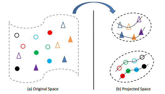
To perform cross-view learning while exploring supervision knowledge in terms of similar and dissimilar relationships among instances in each view and across the views, as well as sample distribution manifolds, we construct DCLMP. To this end, we should construct the model by taking into account the following aspects: 1) distances between similar instances from the same class should be reduced while those among dissimilar from different classes should be enlarged, in levels of intra-view and inter-view; 2) manifold structures embedded in similar and dissimilar instances should be preserved. These modelling considerations are intuitively demonstrated in Figure 1.

Along this line, we construct the objective function of DCLMP as follows:

where ${\textbf U}$ and ${\textbf V}$ denote the projection matrices in the $r$-dimensional common space of two views and $k_{n}$ denotes the $k$-nearest neighbors of an instance. ${\textbf L}$ is the discriminative weighting matrix. ${\textbf S}^{w_x}$ and ${\textbf S}^{w_y}$ stand for the within-class manifold weighting matrices of two different views of feature representations, and ${\textbf S}^{b_x}$ and ${\textbf S}^{b_y}$ stand for the between-class manifold weighting matrices of two different views of feature representations. Their elements are defined as follows

where KNN$_{k_n}$ denotes the $k_n$-nearest neighbors of an instance. $\sigma_x$ and $\sigma_y$ stand for width coefficients to normalize the weights.

In Eq (3.1), the first part characterizes the cross-view similarity and dissimilarity discriminations, the second part preserves the manifold relationships within each class scatters, while the third part magnifies the distribution margins for a dissimilar pair of instances. In this way, both the discriminative information and the manifold distributions can be modelled in a joint objective function.

For convenience of solving Eq (3.1), we transform it as the following concise form

with

where ${\textbf M}^{w_x}_{ii} = \sum_{j = 1}^{N}{\textbf S}_{ij}^{w_x}$, ${\textbf M}^{w_y}_{ii} = \sum_{j = 1}^{N}{\textbf S}_{ij}^{w_y}$, ${\textbf M}^{b_x}_{ii} = \sum_{j = 1}^{N}{\textbf S}_{ij}^{b_x}$, ${\textbf M}^{b_y}_{ii} = \sum_{j = 1}^{N}{\textbf S}_{ij}^{b_y}$, and ${\textbf M}^{L}_{ii} = \sum_{j = 1}^{N}{\textbf L}_{ij}$.

We let $\mathcal{J}$ record the objective function value of Eq (3.7) and introduce ${\textbf Q}^T{\textbf Q} = {\textbf I}$ to replace ${\textbf A}$ and ${\Lambda}$ to rewrite Eq (3.7) as

Calculating the partial derivative of $\mathcal{J}_{\{{\textbf Q}, {\Lambda}\}}$ with regard to Q and making it to zero yields

The projection matrix ${\textbf Q}$ can be obtained by calculating a required number of smallest eigenvectors of ${\textbf C}+\lambda_1 {\textbf S}_z - \lambda_2 {\textbf D}_z$. Finally, we can recover ${\textbf A} = {\textbf Q}{\textbf Q}^T$. Then, ${\textbf U}$ and ${\textbf V}$ can be obtained through Eq (3.8).

3.2.   C-DCLMP

We find that such a objective function may be not convex ^[32,33]. The separability of nonlinear data patterns in the geodesic space can be significantly improved and thus benefits their subsequent recognitions. Referring to $\min_{{\textbf A}\succ 0} \; tr({\textbf A}^{-1}\bullet) \Leftrightarrow \max_{{\textbf A} \succ 0} \; tr({\textbf A}\bullet)$ ^[34], we reformulate DCLMP in (3.7) equivalently as

Minimizing the third term $\lambda_1 tr({\textbf A}^{-1}{\textbf D}_z)$ is equivalent to minimizing $-\lambda_1 tr\left({\textbf AD}_z\right)$ of Eq (3.7). Although the last term is nonlinear, it is defined in the convex cone space ^[35] and thus is still convex. As a result, Eq (3.14) is entirely convex regarding $A$. It enjoys closed-form solution ^[36,37,38]. To distinguish Eq (3.14) from DCLMP, we call it C-DCLMP.

For convenience of deriving the closed-form solution, we reformulate Eq (3.14) as

where we set $\gamma \in (0, 1)$ ^[34]. Let $J({\textbf A}): = \gamma tr({\textbf A}^{-1}{\textbf D}_z) + (1-\gamma)\left(tr\left({\textbf AS}_z\right) + \alpha tr\left({\textbf AC}\right)\right)$.

whose solution is the midpoint of the geodesic jointing $((1-\gamma)({\textbf S}_z+\alpha{\textbf C}))^{-1}$ and $\gamma{\textbf D}_z$, that is

$(\cdot)\sharp_{1/2}(\cdot)$ denotes the midpoint. We extend the geodesic mean solution (3.17) to the geodesic space by replacing $(\cdot)\sharp_{1/2}(\cdot)$ with $(\cdot)\sharp_{t}(\cdot)$, $0\leqslant t\leqslant 1$.

We add a regularizer with prior knowledge to (3.15). Here, we incorporate symmetrized LogDet divergence and consequently (3.15) becomes

where $(p$+$q)$ is the dimension of the data. Fortunately, complying with the definition of geometric mean ^[36], Eq (3.18) is still convex. We let $G({\textbf A}): = \gamma tr({\textbf A}^{-1}{\textbf D}_z) + (1-\gamma)(tr\left({\textbf AS}_z\right) + \alpha tr\left({\textbf AC}\right)) + \lambda D_{sld}({\textbf A}, {\textbf A}_0)$. Then we set the gradient of $G({\textbf A})$ regarding to ${\textbf A}$ to zero and obtain the equation as

we calculate the closed-form solution as

More precisely, according to the definition of $(\cdot)\sharp_{t}(\cdot)$, namely the geodesic mean jointing two matrices, we can directly expand the final solution of our C-DCLMP in Eq (3.18) as

where we set ${\textbf A}_0$ to be a $(p$+$q)$-order identity matrix ${\textbf I}_{p+q}$. When obtaining ${\textbf A}$, ${\textbf U}$ and ${\textbf V}$ are recovered.

Its concatenated representation can be generated by ${\textbf U}^T{\textbf x}+{\textbf V}^T{\textbf y} = \left[\begin{aligned} {\textbf U} \\ {\textbf V} \end{aligned} \right]^T\left[\begin{aligned} {\textbf x}\\ {\textbf y} \end{aligned} \right]$ and the classification decision using a classifier (e.g., KNN) can be made on this fused representation.

4.   Experiment

To comprehensively evaluate the proposed methods, we first performed comparative experiments on several benchmark and real face datasets. Besides, we also performed sensibility analysis on the model parameters.

4.1.   Setup

For evaluation and comparisons, CCA ^[1], DCCA ^[12], MPECCA ^[14], CECCA ^[17], DCA ^[20] and CDCA ^[26] were implemented. All hyper-parameters were cross-validated in the range of [0, 0.1, ..., 1] for $t$ and $\gamma$, and [1e-7, 1e-6, ..., 1e3] for $\alpha$ and $\lambda$. For concatenated cross-view representations, a $5$-nearest-neighbors classifier was employed for classification. Additionally, recognition accuracy (%, higher is better) and mean absolute errors (MAE, lower is better) were adopted as performance measures.

4.2.   Comparisons on non-face datasets

We first performed experiments on several widely used non-face multi-view datasets, i.e., MFD ^[39] and USPS ^[40], AWA ^[41] and ADNI ^[42]. We report the results in Table 1.

The proposed DCLMP method yielded the second-lowest estimation errors in most cases, slightly higher than the proposed C-DCLMP. The improvement achieved by C-DCLMP method is significant, especially on AWA and USPS datasets.

4.3.   Comparisons on face datasets

We also conducted age estimation experiments on AgeDB ^[43], CACD ^[44] and IMDB-WIKI ^[45]. These three databases are illustrated in Figure 2.

We extracted BIF ^[46] and HoG ^[47] feature vectors and reduced dimensions to 200 by PCA as two view representations. We randomly chose 50,100,150 samples for training. Also, we use VGG19 ^[48] and Resnet50 ^[45] to extract deep feature vectors from AgeDB, CACD and IMDB-WIKI databases. We report results in Tables 3, 5 and 6.

The estimation errors (MAEs) of all the methods reduced monotonically. The age MAEs of DCLMP are the second lowest, demonstrating the solidness of our modelling cross-view discriminative knowledge and data manifold structures. We can also observe that C-DCLMP yields the lowest estimation errors, demonstrating its effectiveness and superiority.

4.4.   Parameters analysis

For the proposed methods, we performed parameter analysis $t$, $\gamma$ and $\lambda$ involved in (3.21), respectively. Specifically, we conducted age estimation experiments on both AgeDB and CACD. The results are plotted in Figures 3–5.

Geometric weighting parameter $t$ of C-DCLMP: We find some interesting observations from Figure 3. That is, with $t$ increasing from 0 to 1, the estimation error descended first and then rose again. It shows that the similar manifolds within class and the inter-class data distributions are helpful in regularizing the model solution space.

Metric balance parameter $\gamma$ of C-DCLMP: We can observe from Figure 4 that, the age estimation error (MAE) achieved the lowest values when $0.1 < \gamma < 0.9$. This observation illustrates that preserving the data cross-view discriminative knowledge and the manifold distributions is useful and helps improve the estimation precision.

Metric prior parameter $\lambda$ of C-DCLMP: Figure 5 shows that, with increased $\lambda$ value, age estimation error descended to its lowest around $\lambda$ = 1e-1 and then increased steeply. It demonstrates that incorporating moderate metric prior knowledge can regularize the model solution positively, but excess prior knowledge may dominate the entire data rule and mislead the training of the model.

4.5.   Time complexity analysis

For the proposed methods and the comparison methods mentioned above, we performed time complexity analysis. Specifically, we conducted age estimation experiments on both AgeDB and CACD by choosing 100 samples from each class for training while taking the rest for testing, respectively. We reported the averaged results in Table 7.

4.6.   Ablation experiments

For the proposed methods, we performed ablation experiments. Specifically, we conducted age estimation experiments on both AgeDB and CACD. We repeated the experiment 10 times with random data partitions and reported the averaged results in Table 8. In Table 8, each referred part corresponds to Eq (3.7).

5.   Conclusion

In this paper, we proposed a DCLMP, in which both the cross-view discriminative information and the spatial structural information of training data is taken into consideration to enhance subsequent decision making. To pursue closed-form solutions, we remodeled the objective of DCLMP to nonlinear geodesic space and consequently achieved its convex formulation (C-DCLMP). Finally, we evaluated the proposed methods and demonstrated their superiority on various benchmark and real face datasets. In the future, we will consider exploring the latent information of the unlabeled data from the feature and label level, and study how to combine related advanced multi-view learning methods to reduce the computational consumption of the model and further improve the generalization ability of the model in various scenarios.

Use of AI tools declaration

The authors declare they have not used Artificial Intelligence (AI) tools in the creation of this article.

Acknowledgments

This work was supported by the National Natural Science Foundation of China under Grant 62176128, the Open Projects Program of State Key Laboratory for Novel Software Technology of Nanjing University under Grant KFKT2022B06, the Fundamental Research Funds for the Central Universities No. NJ2022028, the Project Funded by the Priority Academic Program Development of Jiangsu Higher Education Institutions (PAPD) fund, as well as the Qing Lan Project of the Jiangsu Province.