Deep Grassmannian multiview subspace clustering with contrastive learning

Rui Wang; Haiqiang Li; Chen Hu; Xiao-Jun Wu; Yingfang Bao; Rui Wang; Haiqiang Li; Chen Hu; Xiao-Jun Wu; Yingfang Bao

doi:10.3934/era.2024252

Electronic Research Archive

2024, Volume 32, Issue 9: 5424-5450. doi: 10.3934/era.2024252

Previous Article Next Article

Research article

Deep Grassmannian multiview subspace clustering with contrastive learning

1.
School of Artificial Intelligence and Computer Science, Jiangnan University, Wuxi 214122, China
2.
Jiangsu Provincial Engineering Laboratory of Pattern Recognition and Computational Intelligence, Jiangnan University, Wuxi 214122, China
3.
Affiliated Wuxi Fifth Hospital of Jiangnan University, Wuxi 214007, China
4.
The Fifth People's Hospital of Wuxi, Wuxi 214007, China

Received: 25 June 2024 Revised: 13 September 2024 Accepted: 20 September 2024 Published: 26 September 2024

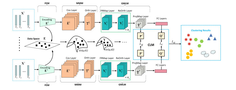
This paper investigated the problem of multiview subspace clustering, focusing on feature learning with submanifold structure and exploring the invariant representations of multiple views. A novel approach was proposed in this study, termed deep Grassmannian multiview subspace clustering with contrastive learning (DGMVCL). The proposed algorithm initially utilized a feature extraction module (FEM) to map the original input samples into a feature subspace. Subsequently, the manifold modeling module (MMM) was employed to map the aforementioned subspace features onto a Grassmannian manifold. Afterward, the designed Grassmannian manifold network was utilized for deep subspace learning. Finally, discriminative cluster assignments were achieved utilizing a contrastive learning mechanism. Extensive experiments conducted on five benchmarking datasets demonstrate the effectiveness of the proposed method. The source code is available at https://github.com/Zoo-LLi/DGMVCL.
- multiview clustering,
- contrastive learning,
- Grassmannian manifold,
- neural network,
- invariant representation
Citation: Rui Wang, Haiqiang Li, Chen Hu, Xiao-Jun Wu, Yingfang Bao. Deep Grassmannian multiview subspace clustering with contrastive learning[J]. Electronic Research Archive, 2024, 32(9): 5424-5450. doi: 10.3934/era.2024252

Related Papers:

Abstract

This paper investigated the problem of multiview subspace clustering, focusing on feature learning with submanifold structure and exploring the invariant representations of multiple views. A novel approach was proposed in this study, termed deep Grassmannian multiview subspace clustering with contrastive learning (DGMVCL). The proposed algorithm initially utilized a feature extraction module (FEM) to map the original input samples into a feature subspace. Subsequently, the manifold modeling module (MMM) was employed to map the aforementioned subspace features onto a Grassmannian manifold. Afterward, the designed Grassmannian manifold network was utilized for deep subspace learning. Finally, discriminative cluster assignments were achieved utilizing a contrastive learning mechanism. Extensive experiments conducted on five benchmarking datasets demonstrate the effectiveness of the proposed method. The source code is available at https://github.com/Zoo-LLi/DGMVCL.

References

[1]	M. C. Tsakiris, R. Vidal, Algebraic clustering of affine subspaces, IEEE Trans. Pattern Anal. Mach. Intell., 40 (2017), 482–489. https://doi.org/10.1109/TPAMI.2017.2678477 doi: 10.1109/TPAMI.2017.2678477
[2]	C. You, C. G. Li, D. P. Robinson, R. Vidal, Is an affine constraint needed for affine subspace clustering?, in Proceedings of the IEEE/CVF International Conference on Computer Vision, (2019), 9915–9924.
[3]	P. Ji, M. Salzmann, H. Li, Shape interaction matrix revisited and robustified: Efficient subspace clustering with corrupted and incomplete data, in Proceedings of the IEEE International Conference on computer Vision, (2015), 4687–4695.
[4]	J. Yang, J. Liang, K. Wang, P. L. Rosin, M. H. Yang, Subspace clustering via good neighbors, IEEE Trans. Pattern Anal. Mach. Intell., 42 (2019), 1537–1544. https://doi.org/10.1109/TPAMI.2019.2913863 doi: 10.1109/TPAMI.2019.2913863
[5]	A. Gruber, Y. Weiss, Multibody factorization with uncertainty and missing data using the EM algorithm, in Proceedings of the 2004 IEEE Computer Society Conference on Computer Vision and Pattern Recognition, (2004), 1–1. https://doi.org/10.1109/CVPR.2004.1315101
[6]	S. R. Rao, R. Tron, R. Vidal, Y. Ma, Motion segmentation via robust subspace separation in the presence of outlying, incomplete, or corrupted trajectories, in 2008 IEEE Conference on Computer Vision and Pattern Recognition, (2008), 1–8. https://doi.org/10.1109/CVPR.2008.4587437
[7]	E. Elhamifar, R. Vidal, Sparse subspace clustering: Algorithm, theory, and applications, IEEE Trans. Pattern Anal. Mach. Intell., 35 (2013), 2765–2781. https://doi.org/10.1109/TPAMI.2013.57 doi: 10.1109/TPAMI.2013.57
[8]	Z. Kang, G. Shi, S. Huang, W. Chen, X. Pu, J. T. Zhou, et al., Multi-graph fusion for multi-view spectral clustering, Knowl.-Based Syst., 189 (2020), 105102. https://doi.org/10.1016/j.knosys.2019.105102 doi: 10.1016/j.knosys.2019.105102
[9]	G. Liu, Z. Lin, S. Yan, J. Sun, Y. Yu, Y. Ma, Robust recovery of subspace structures by low-rank representation, IEEE Trans. Pattern Anal. Mach. Intell., 35 (2012), 171–184. https://doi.org/10.1109/TPAMI.2012.88 doi: 10.1109/TPAMI.2012.88
[10]	J. Shi, J. Malik, Normalized cuts and image segmentation, IEEE Trans. Pattern Anal. Mach. Intell., 22 (2000), 888–905. https://doi.org/10.1109/34.868688 doi: 10.1109/34.868688
[11]	J. Guo, Y. Sun, J. Gao, Y. Hu, B. Yin, Low rank representation on product grassmann manifolds for multi-view subspace clustering, in 2020 25th International Conference on Pattern Recognition (ICPR), (2021), 907–914. https://doi.org/10.1109/ICPR48806.2021.9412242
[12]	W. B. Hu, X. J. Wu, Multi-geometric sparse subspace clustering, Neural Process. Lett., 52 (2020), 849–867. https://doi.org/10.1007/s11063-020-10274-z doi: 10.1007/s11063-020-10274-z
[13]	D. Wei, X. Shen, Q. Sun, X. Gao, Discrete metric learning for fast image set classification, IEEE Trans. Image Process., 31 (2022), 6471–6486. https://doi.org/10.1109/TIP.2022.3212284 doi: 10.1109/TIP.2022.3212284
[14]	G. Cheng, C. Yang, X. Yao, L. Guo, J. Han, When deep learning meets metric learning: Remote sensing image scene classification via learning discriminative CNNs, IEEE Trans. Geosci. Remote Sens., 56 (2018), 2811–2821. https://doi.org/10.1109/TGRS.2017.2783902 doi: 10.1109/TGRS.2017.2783902
[15]	K. Song, J. Han, G. Cheng, J. Lu, F. Nie, Adaptive neighborhood metric learning, IEEE Trans. Pattern Anal. Mach. Intell., 44 (2021), 4591–4604.
[16]	P. Ji, T. Zhang, H. Li, M. Salzmann, I. Reid, Deep subspace clustering networks, Adv. Neural Inf. Process. Syst., 30 (2017).
[17]	H. Wang, Q. Wang, Q. Miao, X. Ma, Joint learning of data recovering and graph contrastive denoising for incomplete multi-view clustering, Inf. Fusion, 104 (2024), 102155. https://doi.org/10.1016/j.inffus.2023.102155 doi: 10.1016/j.inffus.2023.102155
[18]	W. Wu, X. Ma, Q. Wang, M. Gong, Q. Gao, Learning deep representation and discriminative features for clustering of multi-layer networks, Neural Networks, 170 (2024), 405–416. https://doi.org/10.1016/j.neunet.2023.11.053 doi: 10.1016/j.neunet.2023.11.053
[19]	J. Xu, Y. Ren, G. Li, L. Pan, C. Zhu, Z. Xu, Deep embedded multi-view clustering with collaborative training, Inf. Sci., 573 (2021). 279–290. https://doi.org/10.1016/j.ins.2020.12.073 doi: 10.1016/j.ins.2020.12.073
[20]	H. Wang, W. Zhang, X. Ma, Contrastive and adversarial regularized multi-level representation learning for incomplete multi-view clustering, Neural Networks, 172 (2024), 106102. https://doi.org/10.1016/j.neunet.2024.106102 doi: 10.1016/j.neunet.2024.106102
[21]	Y. Yang, X. Ma, Graph contrastive learning for clustering of multi-layer networks, IEEE Trans. Big Data, 2023 (2023). https://doi.org/10.1109/TBDATA.2023.3343349
[22]	W. Guo, H. Che, M. F. Leung, Z. Yan, Adaptive multi-view subspace learning based on distributed optimization, Int. Things, 26 (2024), 101203. https://doi.org/10.1016/j.iot.2024.101203 doi: 10.1016/j.iot.2024.101203
[23]	Z. Li, Q. Wang, Z. Tao, Q. Gao, Z. Yang, Deep adversarial multi-view clustering network, in Proceedings of the Twenty-Eighth International Joint Conference on Artificial Intelligence, 2 (2019), 4.
[24]	H. Ma, W. Wu, A deep clustering framework integrating pairwise constraints and a VMF mixture model, Electron. Res. Arch., 32 (2024), 3952–3972. https://dx.doi.org/10.3934/era.2024177 doi: 10.3934/era.2024177
[25]	Z. Chen, T. Xu, X. J. Wu, R. Wang, Z. Huang, J. Kittler, Riemannian local mechanism for spd neural networks, in Proceedings of the AAAI Conference on Artificial Intelligence, 37 (2023), 7104–7112. https://doi.org/10.1609/aaai.v37i6.25867
[26]	R. Wang, X. J. Wu, Z. Chen, C. Hu, J Kittler Spd manifold deep metric learning for image set classification, IEEE Trans. Neural Networks Learn. Syst., 35 (2024), 8924–8938. https://doi.org/10.1109/TNNLS.2022.3216811 doi: 10.1109/TNNLS.2022.3216811
[27]	T. Liu, Z. Shi, Y. Liu, Visual clustering based on kernel sparse representation on grassmann manifolds, in 2017 IEEE 7th Annual International Conference on CYBER Technology in Automation, Control, and Intelligent Systems (CYBER), (2017), 920–925. https://doi.org/10.1109/CYBER.2017.8446507
[28]	R. Wang, X. J. Wu, Z. Liu, J. Kittler, Geometry-aware graph embedding projection metric learning for image set classification, IEEE Trans. Cognitive Dev. Syst., 14 (2022), 957–970. https://doi.org/10.1109/TCDS.2021.3086814 doi: 10.1109/TCDS.2021.3086814
[29]	R. Wang, X. J. Wu, J. Kittler, Graph embedding multi-kernel metric learning for image set classification with Grassmannian manifold-valued features, IEEE Trans. Multimedia, 23 (2021), 228–242. https://doi.org/10.1109/TMM.2020.2981189 doi: 10.1109/TMM.2020.2981189
[30]	R. Wang, X. J. Wu, T. Xu, C. Hu, J. Kittler, U-SPDNet: An SPD manifold learning-based neural network for visual classification, Neural networks, 161 (2023), 382–396. https://doi.org/10.1016/j.neunet.2022.11.030 doi: 10.1016/j.neunet.2022.11.030
[31]	K. X. Chen, X. J. Wu, R. Wang, J. Kittler, Riemannian kernel based Nyström method for approximate infinite-dimensional covariance descriptors with application to image set classification, in 2018 24th International Conference on Pattern Recognition (ICPR), (2018), 651–656. https://doi.org/10.1109/ICPR.2018.8545822
[32]	T. Bendokat, R. Zimmermann, P. A. Absil, A grassmann manifold handbook: Basic geometry and computational aspects, Adv. Comput. Math., 50 (2024), 1–51. https://doi.org/10.1007/s10444-023-10090-8 doi: 10.1007/s10444-023-10090-8
[33]	D. Wei, X. Shen, Q. Sun, X. Gao, Z. Ren, Sparse representation classifier guided Grassmann reconstruction metric learning with applications to image set analysis, IEEE Trans. Multimedia, 25 (2022), 4307–4322. https://doi.org/10.1109/TMM.2022.3173535 doi: 10.1109/TMM.2022.3173535
[34]	B. Wang, Y. Hu, J. Gao, Y. Sun, B. Yin, Low rank representation on Grassmann manifolds, in Computer Vision–ACCV 2014: 12th Asian Conference on Computer Vision, (2015), 81–96. https://doi.org/10.1007/978-3-319-16865-4_6
[35]	X. Piao, Y. Hu, J. Gao, Y. Sun, B. Yin, Double nuclear norm based low rank representation on Grassmann manifolds for clustering, in Proceedings of the IEEE/CVF Conference on Computer Vision and Pattern Recognition, (2019), 12075–12084.
[36]	C. Zhang, Q. Hu, H. Fu, P. Zhu, X. Cao, Latent multi-view subspace clustering, in Proceedings of the IEEE Conference on Computer Vision and Pattern Recognition, (2017), 4279–4287.
[37]	R. Li, C. Zhang, Q. Hu, P. Zhu, Z. Wang, Flexible multi-view representation learning for subspace clustering, in Proceedings of the Twenty-Eighth International Joint Conference on Artificial Intelligence, (2019), 2916–2922.
[38]	R. Zhou, Y. D. Shen, End-to-end adversarial-attention network for multi-modal clustering, in Proceedings of the IEEE/CVF Conference on Computer Vision and Pattern Recognition, (2020), 14619–14628.
[39]	Z. Kang, Z. Lin, X. Zhu, W. Xu, Structured graph learning for scalable subspace clustering: From single view to multiview, IEEE Trans. Cybern., 52 (2021), 8976–8986. https://doi.org/10.1109/TCYB.2021.3061660 doi: 10.1109/TCYB.2021.3061660
[40]	E. Pan, Z. Kang, High-order multi-view clustering for generic data, Inf. Fusion, 100 (2023), 101947. https://doi.org/10.1016/j.inffus.2023.101947 doi: 10.1016/j.inffus.2023.101947
[41]	J. Chen, S. Yang, X. Peng, D. Peng, Z. Wang, Augmented sparse representation for incomplete multiview clustering, IEEE Trans. Neural Networks Learn. Syst., 35 (2022), 4058–4071. https://doi.org/10.1109/TNNLS.2022.3201699 doi: 10.1109/TNNLS.2022.3201699
[42]	T. Chen, S. Kornblith, M. Norouzi, G. Hinton, A simple framework for contrastive learning of visual representations, in International Conference on Machine Learning, (2020), 1597–1607.
[43]	Y. Tian, C. Sun, B. Poole, D. Krishnan, C. Schmid, P. Isola, What makes for good views for contrastive learning?, Adv. Neural Inf. Process. Syst., 33 (2020), 6827–6839.
[44]	T. Wang, P. Isola, Understanding contrastive representation learning through alignment and uniformity on the hypersphere, in International Conference on Machine Learning, (2020), 9929–9939.
[45]	M. Harandi, C. Sanderson, C. Shen, B. C. Lovell, Dictionary learning and sparse coding on Grassmann manifolds: An extrinsic solution, in Proceedings of the IEEE International Conference on Computer Vision (ICCV), (2013), 3120–3127.
[46]	Z. Huang, J. Wu, L. Van Gool, Building deep networks on Grassmann manifolds, in Proceedings of the AAAI Conference on Artificial Intelligence, (2018), 1137–1145. https://doi.org/10.1609/aaai.v32i1.11725
[47]	A. Edelman, T. A. Arias, S. T. Smith, The geometry of algorithms with orthogonality constraints, SIAM J. Matrix Anal. Appl., (1998), 303–353. https://doi.org/10.1137/S0895479895290954
[48]	P. A. Absil, R. Mahony, R. Sepulchre, Optimization Algorithms on Matrix Manifolds, Princeton University Press, 2009.
[49]	J. Hamm, D. D. Lee, Grassmann discriminant analysis: A unifying view on subspace-based learning, in Proceedings of the 25th International Conference on Machine Learning, (2008), 376–383. https://doi.org/10.1145/1390156.1390204
[50]	J. Hamm, D. Lee, Extended Grassmann kernels for subspace-based learning, Adv. Neural Inf. Process. Syst., (2008), 21.
[51]	M. T. Harandi, C. Sanderson, S. Shirazi, B. C. Lovell, Graph embedding discriminant analysis on Grassmannian manifolds for improved image set matching, in CVPR 2011, (2011), 2705–2712. https://doi.org/10.1109/CVPR.2011.5995564
[52]	Z. Huang, S. Shan, R. Wang, H. Zhang, S. Lao, A. Kuerban, et al., A benchmark and comparative study of video-based face recognition on cox face database, IEEE Trans. Image Process., 24 (2015), 5967–5981. https://doi.org/10.1109/TIP.2015.2493448 doi: 10.1109/TIP.2015.2493448
[53]	C. Cui, Y. Ren, J. Pu, X. Pu, L. He, Deep multi-view subspace clustering with anchor graph, preprint, arXiv: 2305.06939. https://doi.org/10.48550/arXiv.2305.06939
[54]	P. Xia, L. Zhang, F. Li, Learning similarity with cosine similarity ensemble, Inf. Sci., 307 (2015), 39–52. https://doi.org/10.1016/j.ins.2015.02.024 doi: 10.1016/j.ins.2015.02.024
[55]	J. Chen, H. Mao, W. L. Woo, X. Peng, Deep multiview clustering by contrasting cluster assignments, in Proceedings of the IEEE/CVF International Conference on Computer Vision, (2023), 16752–16761.
[56]	A. Asuncion, D. Newman, UCI Machine Learning Repository, 2007. Available from: https://ergodicity.net/2013/07/
[57]	J. Xu, Y. Ren, H. Tang, X. Pu, X. Zhu, M. Zeng, et al., Multi-VAE: Learning disentangled view-common and view-peculiar visual representations for multi-view clustering, in Proceedings of the IEEE/CVF International Conference on Computer Vision, (2021), 9234–9243.
[58]	H. Xiao, K. Rasul, R. Vollgraf, Fashion-mnist: A novel image dataset for benchmarking machine learning algorithms, preprint, arXiv: 1708.07747. https://doi.org/10.48550/arXiv.1708.07747
[59]	M. D. Addlesee, A. Jones, F. Livesey, F. Samaria, The ORL active floor [sensor system], IEEE Pers. Commun., 4 (1997), 35–41. https://doi.org/10.1109/98.626980 doi: 10.1109/98.626980
[60]	F. F. Li, P. Perona, A bayesian hierarchical model for learning natural scene categories, in 2005 IEEE Computer Society Conference on Computer Vision and Pattern Recognition (CVPR'05), 2 (2005), 524–531. https://doi.org/10.1109/CVPR.2005.16
[61]	U. Von Luxburg, A tutorial on spectral clustering, Stat. Comput., 17 (2007), 395–416. https://doi.org/10.1007/s11222-007-9033-z doi: 10.1007/s11222-007-9033-z
[62]	F. Nie, X. Wang, H. Huang, Clustering and projected clustering with adaptive neighbors, in Proceedings of the 20th ACM SIGKDD International Conference on Knowledge Discovery and Data Mining, (2014), 977–986. https://doi.org/10.1145/2623330.2623726
[63]	H. Tang, Y. Liu, Deep safe incomplete multi-view clustering: Theorem and algorithm, in International Conference on Machine Learning, (2022), 21090–21110.
[64]	Y. Lin, Y. Gou, X. Liu, J. Bai, J. Lv, X. Peng, Dual contrastive prediction for incomplete multi-view representation learning, IEEE Trans. Pattern Anal. Mach. Intell., 45 (2022), 4447–4461. https://doi.org/10.1109/TPAMI.2022.3197238 doi: 10.1109/TPAMI.2022.3197238
[65]	J. Xu, H. Tang, Y. Ren, L. Peng, X. Zhu, L. He, Multi-level feature learning for contrastive multi-view clustering, in Proceedings of the IEEE/CVF Conference on Computer Vision and Pattern Recognition, (2022), 16051–16060.
[66]	L. Van der Maaten, G. Hinton, Visualizing data using t-SNE., J. Mach. Learn. Res., 9 (2008).
[67]	Y. Cai, H. Che, B. Pan, M. F. Leung, C. Liu, S. Wen, Projected cross-view learning for unbalanced incomplete multi-view clustering, Inf. Fusion, 105 (2024), 102245. https://doi.org/10.1016/j.inffus.2024.102245 doi: 10.1016/j.inffus.2024.102245
[68]	K. He, X. Zhang, S. Ren, J. Sun, Deep residual learning for image recognition, inn Proceedings of the IEEE Conference on Computer Vision and Pattern Recognition (CVPR), (2016), 770–778.

Reader Comments

Your name:*

Email:*
© 2024 the Author(s), licensee AIMS Press. This is an open access article distributed under the terms of the Creative Commons Attribution License (http://creativecommons.org/licenses/by/4.0)