Recently, TechCrunch, a digital economy news site, noted that "Uber, the world's largest taxi company, owns no vehicles. Facebook, the world's most popular media owner, creates no content. Alibaba, the most valuable retailer, has no inventory. And Airbnb, the world's largest accommodation provider, owns no real estate, something interesting is happening." All these companies are involved in e-commerce business, namely the process of buying and selling products by electronic means, such as mobile applications and the Internet. In light of this, this study aimed to examine the relationship between e-commerce and digital economy, with a particular focus on the mediating role of customers' attitudes. To achieve this objective, the study employed a mixed research approach and adopted an explanatory research design. The target population consisted of all customers who are potential e-commerce users. Convenience sampling techniques were employed to collect data from respondents. The findings of the study revealed a positive and significant relationship between e-commerce and the digital economy, both in terms of direct and indirect effects. Additionally, the study identified the partial mediating role of customer attitudes in this relationship. Based on these findings, the study recommends that e-commerce companies should explore the potential of social networking media platforms such as Facebook and Instagram to further enhance overall e-commerce usage among customers. This strategic approach can complement their existing platforms and contribute to their growth and success in the digital economy.
Citation: Goshu Desalegn, Anita Tangl, Anita Boros. The mediating role of customer attitudes in the linkage between e-commerce and the digital economy[J]. National Accounting Review, 2024, 6(2): 245-265. doi: 10.3934/NAR.2024011
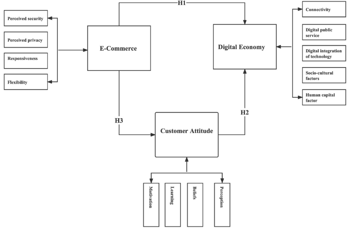
Recently, TechCrunch, a digital economy news site, noted that "Uber, the world's largest taxi company, owns no vehicles. Facebook, the world's most popular media owner, creates no content. Alibaba, the most valuable retailer, has no inventory. And Airbnb, the world's largest accommodation provider, owns no real estate, something interesting is happening." All these companies are involved in e-commerce business, namely the process of buying and selling products by electronic means, such as mobile applications and the Internet. In light of this, this study aimed to examine the relationship between e-commerce and digital economy, with a particular focus on the mediating role of customers' attitudes. To achieve this objective, the study employed a mixed research approach and adopted an explanatory research design. The target population consisted of all customers who are potential e-commerce users. Convenience sampling techniques were employed to collect data from respondents. The findings of the study revealed a positive and significant relationship between e-commerce and the digital economy, both in terms of direct and indirect effects. Additionally, the study identified the partial mediating role of customer attitudes in this relationship. Based on these findings, the study recommends that e-commerce companies should explore the potential of social networking media platforms such as Facebook and Instagram to further enhance overall e-commerce usage among customers. This strategic approach can complement their existing platforms and contribute to their growth and success in the digital economy.

| [1] |
Armstrong JS, Overton TS (1977) Estimating nonresponse bias in mail surveys. J Mark Res 14: 396–402. https://doi.org/10.1177/002224377701400320 doi: 10.1177/002224377701400320

|
| [2] | Abid M, Shah H, Arafa A, et al. (2021) Plurilateral negotiation of WTO E-commerce in the context of digital economy: recent issues and developments. J Law Polit Sci 26: 28–54. |
| [3] | Alam MI, Gani MO (2019) Determinants of omnichannel customer experience: A growing digital economy perspective. J Bus 40: 203–230. |
| [4] | ALraja MN, Aref M (2015) Customer acceptance of e-commerce: integrating perceived risk with TAM. Int J Appl Bus Econ Res 13: 913–921. |
| [5] |
Ardiansah MN, Chariri A, Januarti I (2019) Empirical study on customer perception of E-commerce: Mediating effect of electronic payment security. J Dinamika Akuntansi 11: 122–131. https://doi.org/10.15294/jda.v11i2.20147 doi: 10.15294/jda.v11i2.20147
|
| [6] | Barnes S, Vidgen R (2002) An integrative approach to the assessment of E-commerce quality. J Electron Commer Res 3: 114–127. |
| [7] |
Bauboniene Z, Guleviciute G (2015) E-commerce factors influencing consumers' online shopping decision. Soc Technol 5: 74–81. https://doi.org/10.13165/ST-15-5-1-06 doi: 10.13165/ST-15-5-1-06
|
| [8] |
Brand MJ, Huizingh EK (2008) Into the drivers of innovation adoption: What is the impact of the current level of adoption? Eur J Innov Manag 11: 5–24. https://doi.org/10.1108/14601060810845204 doi: 10.1108/14601060810845204
|
| [9] | Chai Y, Yu X, Gu X (2018) The concept and framework of basic information facilities for E-commerce. Proceedings - 2018 IEEE 15th International Conference on e-Business Engineering, ICEBE 2018, 312–317. https://doi.org/10.1109/ICEBE.2018.00059 |
| [10] |
Chen YS, Lin CK, Lin CY, et al. (2017) Electronic commerce marketing-based social networks in evaluating competitive advantages using SORM. Int J Soc Humanist Comput 2: 261–277. https://doi.org/10.1504/IJSHC.2017.084760 doi: 10.1504/IJSHC.2017.084760
|
| [11] | Dan W, Song M (2009) Multi-agent systems set for B2B E-commerce systems. 2009 International Conference on Management of e-Commerce and e-Government, ICMeCG 2009, 3–8. https://doi.org/10.1109/ICMeCG.2009.95 |
| [12] |
Dawes J (2008) Do data characteristics change according to the number of scale points used? An experiment using 5-point, 7-point and 10-point scales. Int J Market Res 50: 61–77. https://doi.org/10.1177/147078530805000106 doi: 10.1177/147078530805000106
|
| [13] | De Mendonca CMC, De Andrade AMV (2018) Use of the elements of digital transformation in dynamic capabilities in a Brazilian capital | Uso de Elementos da Transformação Digital nas Capacidades Dinǎmicas em uma Capital Brasileira. Iberian Conference on Information Systems and Technologies, CISTI, 2018-June, 1–6. |
| [14] | Dong Z (2017) E-commerce trend and E-customer analyzing: Online shopping. Oulu University of Applied Sciences. |
| [15] | Eid MI (2011) Determinants of e-commerce customer satisfaction, trust, and loyalty in Saudi Arabia. J Electron Commer Res 12: 78–93. |
| [16] |
Fokina O, Barinov S (2019) Marketing concepts of customer experience in digital economy. E3S Web of Conferences, 135. https://doi.org/10.1051/e3sconf/201913504048 doi: 10.1051/e3sconf/201913504048
|
| [17] |
Frels RK, Onwuegbuzie AJ (2013) Administering quantitative instruments with qualitative interviews: A mixed research approach. J Couns Dev 91: 184–194. https://doi.org/10.1002/j.1556-6676.2013.00085.x doi: 10.1002/j.1556-6676.2013.00085.x
|
| [18] |
Gazieva LR (2021) The impact of E-commerce on the digital economy. Eur Proc Soc Behav Sci, 121–126. https://doi.org/10.15405/epsbs.2021.03.16 doi: 10.15405/epsbs.2021.03.16
|
| [19] |
Gefen D, Rigdon EE, Straub D (2011) An update and extension to SEM guidelines for administrative and Social Science Research. MIS Q 35: iii-xiv. https://doi.org/10.2307/23044042 doi: 10.2307/23044042
|
| [20] |
Gefen D, Straub D (2005) A practical guide to factorial validity using PLS-Graph: tutorial and annotated example. Commun Assoc Inf Syst 16: 91–109. https://doi.org/10.17705/1cais.01605 doi: 10.17705/1cais.01605
|
| [21] |
Hair JF, Risher JJ, Sarstedt M, et al. (2019) When to use and how to report the results of PLS-SEM. Eur Bus Rev 31: 2–24. https://doi.org/10.1108/EBR-11-2018-0203 doi: 10.1108/EBR-11-2018-0203
|
| [22] | Henry D, Cooke S, Buckley P, et al. (1999) The emerging digital economy Ⅱ. Available from: https://www.commerce.gov/sites/default/files/migrated/reports/ede2report_0.pdf. |
| [23] |
Hernandez B, Jimenez J, Martín MJ (2009) Adoption vs acceptance of e-commerce: two different decisions. Eur J Market 43: 1232–1245. https://doi.org/10.1108/03090560910976465 doi: 10.1108/03090560910976465
|
| [24] | Hidiroglou MA, Kim JK, Nambeu CO (2016) A note on regression estimation with unknown population size. Surv Methodol 42: 121–135. |
| [25] | Hox JJ, Boeije HR (2004) Data collection, primary vs. secondary, In: Kempf-Leonard, K., Encyclopedia of Social Measurement, Elsevier, 593–599. https://doi.org/10.1016/B0-12-369398-5/00041-4 |
| [26] |
Jahanshahi AA, Zhang SX, Brem A (2013) E-commerce for SMEs: Empirical insights from three countries. J Small Bus Enterp Dev 20: 849–865. https://doi.org/10.1108/JSBED-03-2012-0039 doi: 10.1108/JSBED-03-2012-0039
|
| [27] |
Jehangir M, Dominic PDD, Naseebullah N, et al. (2011) Towards digital economy: The development of ICT and E-commerce in Malaysia. Mod Appl Sci 5: 171–178. https://doi.org/10.5539/mas.v5n2p171 doi: 10.5539/mas.v5n2p171
|
| [28] | Johnson D, Turner C (2004) International business: Themes and issues in the modern global economy (1st ed.). London: Routledge. https://doi.org/10.4324/9780203634141 |
| [29] |
Kassim N, Asiah NA (2010) The effect of perceived service quality dimensions on customer satisfaction, trust, and loyalty in e-commerce settings: A cross cultural analysis. Asia Pac J Market Logist 22: 351–371. https://doi.org/10.1108/13555851011062269 doi: 10.1108/13555851011062269
|
| [30] | Khan AG (2016) A Study on benefits and challenges in an emerging economy. Glob J Manage Bus Res 16: 26–28. |
| [31] |
Khodaei Valahzaghard M, Bagherzadeh Bilandi E (2014) The impact of electronic banking on profitability and market share: Evidence from banking industry. Manage Sci Lett 4: 2531–2536. https://doi.org/10.5267/j.msl.2014.11.003 doi: 10.5267/j.msl.2014.11.003
|
| [32] | Kinfemichael N (2019) Factors affecting the adoption of e-commerce in tour operators in Ethiopia. Addis Ababa University College of Business & Economics. |
| [33] |
Kiu CC, Lee CS (2017) E-commerce market trends: A case study in leveraging Web 2.0 technologies to gain and improve competitive advantage. Int J Bus Inform Syst 25: 373–392. https://doi.org/10.1504/IJBIS.2017.10005086 doi: 10.1504/IJBIS.2017.10005086
|
| [34] |
Kwadwo M, Martinson A, Evans T, et al. (2016) Barriers to e-commerce adoption and implementation strategy: empirical review of small and medium-sized enterprises in Ghana. Brit J Econ Manage Trade 13: 1–13. https://doi.org/10.9734/bjemt/2016/25177 doi: 10.9734/bjemt/2016/25177
|
| [35] |
Lavrov R, Burkina N, Popovskyi Y, et al. (2020) Customer classification and decision making in the digital economy based on scoring models. Int J Manage 11: 1463–1481. https://doi.org/10.34218/IJM.11.6.2020.134 doi: 10.34218/IJM.11.6.2020.134
|
| [36] |
Lee S, Lee S, Park Y (2007) A prediction model for success of services in e-commerce using decision tree: E-customer's attitude towards online service. Expert Syst Appl 33: 572–581. https://doi.org/10.1016/j.eswa.2006.06.005 doi: 10.1016/j.eswa.2006.06.005
|
| [37] |
Lin B, Shen B (2023) Study of consumers' purchase intentions on community E-commerce platform with the SOR model: a case study of China's "Xiaohongshu" app. Behav Sci 13: 103. https://doi.org/10.3390/bs13020103 doi: 10.3390/bs13020103
|
| [38] | Li H, Zhang Y, Wu J (2013) The future of e-commerce logistics. 2008 IEEE International Conference on Service Operations and Logistics, and Informatics 1: 1403–1408. https://doi.org/10.1109/SOLI.2008.4686621 |
| [39] |
Martinsons MG (2008) Relationship-based e-commerce: Theory and evidence from China. Inf Syst J 18: 331–356. https://doi.org/10.1111/j.1365-2575.2008.00302.x doi: 10.1111/j.1365-2575.2008.00302.x
|
| [40] | Megersa D (2019) School of commerce department of marketing management Addis Ababa University School of commerce department of marketing management post graduate program board of examiners approval sheet the effect of e-commerce on customer loyalty: An empirical study. Available from: http://etd.aau.edu.et/handle/123456789/19922. |
| [41] |
Mentsiev AU, Engel MV, Tsamaev AM, et al. (2020) The concept of digitalization and its impact on the modern eeconomy. Proceedings of the International Scientific Conference "Far East Con" (ISCFEC 2020) 128: 10–15. https://doi.org/10.2991/aebmr.k.200312.422 doi: 10.2991/aebmr.k.200312.422
|
| [42] | Mesenbourgh TL (2001) Measuring Digital Economy. US Bureau of the Census, 1–19. |
| [43] | Mevik BH, Wehrens R (2007) PDF hosted at the Radboud Repository of the Radboud University Nijmegen Article information. J Stat Softw 18: 3–6. |
| [44] |
Michałowska M, Kotylak S, Danielak W (2015) Forming relationships on the e-commerce market as a basis to build loyalty and create value for the customer. Empirical findings. Management 19: 57–72. https://doi.org/10.1515/manment-2015-0005 doi: 10.1515/manment-2015-0005
|
| [45] |
Milewska B (2019) The e-commerce logistics models of Polish clothing companies and their impacts on sustainable development. Scientific Journals of the Maritime University of Szczecin-Zeszyty Naukowe Akademii Morskiej W Szczecinie 60: 140–146. https://doi.org/10.17402/382 doi: 10.17402/382
|
| [46] |
Mohd Thas Thaker H, Khaliq A, Ah Mand A, et al. (2021) Exploring the drivers of social media marketing in Malaysian Islamic banks: An analysis via smart PLS approach. J Islamic Mark 12: 145–165. https://doi.org/10.1108/JIMA-05-2019-0095 doi: 10.1108/JIMA-05-2019-0095
|
| [47] |
Molla A, Heeks R (2007) Exploring e-commerce benefits for businesses in a developing country. Inf Soc 23: 95–108. https://doi.org/10.1080/01972240701224028 doi: 10.1080/01972240701224028
|
| [48] |
Moore RK (2000) Spoken language technology: where do we go from here? Association for Computational Linguistics Ⅰ: 22–22. https://doi.org/10.3115/1075218.1075221 doi: 10.3115/1075218.1075221
|
| [49] |
Palacios JJ (2003) The development of e-commerce in Mexico: A business-led passing boom or a step toward the emergence of a digital economy? Inf Soc 19: 69–79. https://doi.org/10.1080/01972240309479 doi: 10.1080/01972240309479
|
| [50] | Pan CL, Bai X, Li F, et al. (2021) How Business Intelligence Enables E-commerce: Breaking the Traditional E-commerce Mode and Driving the Transformation of Digital Economy. Proceedings - 2nd International Conference on E-Commerce and Internet Technology, ECIT 2021, 26–30. https://doi.org/10.1109/ECIT52743.2021.00013 |
| [51] | Pan CL, Yu Y, Zhou W, et al. (2021) Research on Digitizing and E-commerce in the Era of the Digital Economy. Proceedings - 2nd International Conference on E-Commerce and Internet Technology, ECIT 2021, 189–192. https://doi.org/10.1109/ECIT52743.2021.00050 |
| [52] | Priescu I, Patriciu VV, Nicolaescu S (2009) The viewpoint of E-commerce security in the digital economy. Proceedings - 2009 International Conference on Future Computer and Communication, ICFCC 2009, 431–433. https://doi.org/10.1109/ICFCC.2009.43 |
| [53] |
Qi L, Xu X, Zhang X, et al. (2016) Structural Balance Theory-Based E-Commerce Recommendation over Big Rating Data. IEEE Trans Big Data 4: 301–312. https://doi.org/10.1109/tbdata.2016.2602849 doi: 10.1109/tbdata.2016.2602849
|
| [54] | Qin Z, Chang Y, Li S, et al. (2016) E-Commerce Strategy. https://doi.org/10.1007/978-3-642-39414-0 |
| [55] |
Quinton S, Canhoto A, Molinillo S, et al. (2018) Conceptualising a digital orientation: antecedents of supporting SME performance in the digital economy. J Strateg Mark 26: 427–439. https://doi.org/10.1080/0965254X.2016.1258004 doi: 10.1080/0965254X.2016.1258004
|
| [56] | Rattanawiboonsom V (2016) Effectiveness of critical success factor (CSFs) in electronic supply chain management for Thai manufacturing SMEs industry. POMS 27th Annual Conference, 1–8. Available from: https://www.pomsmeetings.org/ConfProceedings/065/FullPapers/FinalFullPapers/065-1631.pdf. |
| [57] | Sandberg ECW, Håkansson KW (2014) Barriers to adapt eCommerce by rural Microenterprises in Sweden: A case study. Int J Knowl Res Manage E-Commer 4: 1–7. |
| [58] | Sarstedt M, Ringle CM, Hair JF (2020) Partial Least Squares Structural Equation Modeling. In: Homburg, C., Klarmann, M., Vomberg, A. (eds) Handbook of Market Research. Springer, Cham. 587–632. https://doi.org/10.1007/978-3-319-57413-4_15 |
| [59] | Savchenko V (2015) Future Development of E-Commerce in Russia and Germany. Polytechnic University of Valencia Faculty, September, 1–56. |
| [60] | Series E (2015) Electronic Commerce, Part of the Information Society. Analele Universităţii Constantin Brâncuşi Din Târgu Jiu: Seria Economie 1: 78–81. |
| [61] |
Sharma G, Lijuan W (2014) Ethical perspectives on e-commerce: An empirical investigation. Internet Res 24: 414–435. https://doi.org/10.1108/IntR-07-2013-0162 doi: 10.1108/IntR-07-2013-0162
|
| [62] | Singh VP (2005) Digital economy: impacts, influences and challenges. https://doi.org/10.4018/978-1-59140-363-0 |
| [63] | Sirak K (2020) The role of e-commerce in improving supply chain: the case of selected online retail shops in Addis Ababa. Available from https://etd.aau.edu.et/server/api/core/bitstreams/0a226aaa-17a7-4e20-96b7-9ed17bcc2475/content. |
| [64] |
Sirurmath SS (2004) Electronic commerce. Vikalpa 29: 177–185. https://doi.org/10.1177/0256090920040313 doi: 10.1177/0256090920040313
|
| [65] |
Sui DZ, Rejeski DW (2002) Environmental impacts of the emerging digital economy: The e-for-environment e-commerce? Environ Manage 29: 155–163. https://doi.org/10.1007/s00267-001-0027-X doi: 10.1007/s00267-001-0027-X
|
| [66] |
Terzi N (2011) The impact of e-commerce on international trade and employment. Procedia Soc Behav Sci 24: 745–753. https://doi.org/10.1016/j.sbspro.2011.09.010 doi: 10.1016/j.sbspro.2011.09.010
|
| [67] | Unold J (2003) Basic aspects of the digital economy. Available from: https://core.ac.uk/download/pdf/71971973.pdf. |
| [68] |
Volkova N, Kuzmuk I, Oliinyk N, et al. (2021) Development trends of the digital economy: E-business, e-commerce. Int J Comput Sci Netw Secur 21: 186–198. https://doi.org/10.22937/IJCSNS.2021.21.4.23 doi: 10.22937/IJCSNS.2021.21.4.23
|
| [69] |
Wang Y, Sun SJ (2010) Assessing beliefs, attitudes, and behavioral responses toward online advertising in three countries. Int Bus Rev 19: 333–344. https://doi.org/10.1016/j.ibusrev.2010.01.004 doi: 10.1016/j.ibusrev.2010.01.004
|
| [70] | Yang W (2017) Analysis on online payment systems of e-commerce. Available from: https://www.theseus.fi/handle/10024/139600. |
| [71] |
Yapar BK, Bayrakdar S, Yapar M (2015) The role of taxation problems on the development of e-commerce. Procedia Soc Behav Sci 195: 642–648. https://doi.org/10.1016/j.sbspro.2015.06.145 doi: 10.1016/j.sbspro.2015.06.145
|
| [72] | Yehorov Y (2017) The role of e-commerce on sales in selected countries. Available from: http://i-rep.emu.edu.tr:8080/xmlui/bitstream/handle/11129/4924/yehorovyehor.pdf?sequence=1. |
| [73] | Yu H, Huang X, Hu X, et al. (2009) Knowledge management in e-commerce: A data mining perspective. 2009 International Conference on Management of E-Commerce and e-Government, ICMeCG 2009, 152–155. https://doi.org/10.1109/ICMeCG.2009.109 |
| [74] |
Zimmermann HD (2015) Understanding the digital economy: challenges for new business models. SSRN Electron J, 729–732. https://doi.org/10.2139/ssrn.2566095 doi: 10.2139/ssrn.2566095
|
| [75] | Zuroni MJ, Goh HL (2012) Factors influencing consumers' attitude towards e-commerce purchases through online shopping. Int J Humanit Soc Sci 2: 223–230. |
| [76] |
Zhang KZ, Benyoucef M (2016) Consumer behavior in social commerce: A literature review. Decis Support Syst 86: 95–108. https://doi.org/10.1016/j.dss.2016.04.001 doi: 10.1016/j.dss.2016.04.001
|
Figures(1) / Tables(4)

Goshu Desalegn, Anita Tangl, Anita Boros. The mediating role of customer attitudes in the linkage between e-commerce and the digital economy[J]. National Accounting Review, 2024, 6(2): 245-265. doi: 10.3934/NAR.2024011


 DownLoad: