We consider a conical body facing a supersonic stream of air at a uniform velocity. When the opening angle of the obstacle cone is small, the conical shock wave is attached to the vertex. Under the assumption of self-similarity for irrotational motions, the Euler system is transformed into the nonlinear ODE system. We reformulate the problem in a non-dimensional form and analyze the corresponding ODE system. The initial data is given on the obstacle cone and the solution is integrated until the Rankine-Hugoniot condition is satisfied on the shock cone. By applying the fundamental theory of ODE systems and technical estimates, we construct supersonic solutions and also show that no matter how small the opening angle is, a smooth transonic solution always exists as long as the speed of the incoming flow is suitably chosen for this given angle.
Citation: Wen-Ching Lien, Yu-Yu Liu, Chen-Chang Peng. Smooth Transonic Flows Around Cones[J]. Networks and Heterogeneous Media, 2022, 17(6): 827-845. doi: 10.3934/nhm.2022028
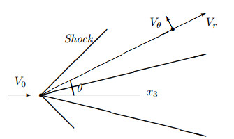
We consider a conical body facing a supersonic stream of air at a uniform velocity. When the opening angle of the obstacle cone is small, the conical shock wave is attached to the vertex. Under the assumption of self-similarity for irrotational motions, the Euler system is transformed into the nonlinear ODE system. We reformulate the problem in a non-dimensional form and analyze the corresponding ODE system. The initial data is given on the obstacle cone and the solution is integrated until the Rankine-Hugoniot condition is satisfied on the shock cone. By applying the fundamental theory of ODE systems and technical estimates, we construct supersonic solutions and also show that no matter how small the opening angle is, a smooth transonic solution always exists as long as the speed of the incoming flow is suitably chosen for this given angle.

| [1] |
J. D. Anderson, Modern Compressible Flow with Historical Perspective, McGraw Hill, 2004. |
| [2] |
L. Bers, Mathematical Aspects of Subsonic and Transonic Gas Dynamics, John Wiley & Sons, Inc., 1958. |
| [3] |
G. W. Bluman and J. D. Cole, Similarity Methods for Differential Equations, Applied Mathematical Sciences, Vol. 13. Springer-Verlag, New York-Heidelberg, 1974. |
| [4] | Drucke auf kegelformige Spitzen bei Bewegung mit Uberschallgeschwindigkei. Z. Angew. Math. Mech. (1929) 9: 496-498. |
| [5] | (2002) Introduction to Symmetry Analysis. Cambridge Univ. Press. |
| [6] |
Stability of transonic shock fronts in three-dimensional conical steady potential flow past a perturbed cone. Discrete Contin. Dyn. Syst. (2009) 23: 85-114. 
|
| [7] | Drag of a Finite Wedge at high subsonic speeds. J. Math. and Physics (1951) 30: 79-92. |
| [8] |
R. Courant and K. O. Friedrichs, Supersonic Flow and Shock Waves, Interscience Publishers, Inc., New York, N. Y. 1948. |
| [9] | (1974) Differential Equations, Dynamical Systems, and Linear Algebra. New York-London: Academic Press. |
| [10] | (1959) Fluid Mechanics. Pergamon Press. |
| [11] |
Nonlinear stability of a self-similar 3-dimensional gas flow. Comm. Math. Phys (1999) 204: 525-549.
|
| [12] |
Self-similar solutions of the Euler Equations with spherical symmetry. Nonlinear Anal. (2012) 75: 6370-6378.
|
| [13] | The air pressure on a cone moving at high speed. Proc. Roy. Soc. (London) Ser A (1933) 139: 278-311. |
| [14] |
G. B. Whitham, Linear and Nonlinear Waves, John Wiley & Sons, New York, 1974. |


Figures(9)
Wen-Ching Lien, Yu-Yu Liu, Chen-Chang Peng. Smooth Transonic Flows Around Cones[J]. Networks and Heterogeneous Media, 2022, 17(6): 827-845. doi: 10.3934/nhm.2022028

Spherical coordinate system
The shock cone
The
The fixed point
The numerical solution for
The numerical result for
List of the symbols
The simulations of shock polars


 DownLoad: