We consider two scalar conservation laws with non-local flux functions, describing traffic flow on roads with rough conditions. In the first model, the velocity of the car depends on an averaged downstream density, while in the second model one considers an averaged downstream velocity. The road condition is piecewise constant with a jump at $ x = 0 $. We study stationary traveling wave profiles cross $ x = 0 $, for all possible cases. We show that, depending on the case, there could exit infinitely many profiles, a unique profile, or no profiles at all. Furthermore, some of the profiles are time asymptotic solutions for the Cauchy problem of the conservation laws under mild assumption on the initial data, while other profiles are unstable.
Citation: Wen Shen. Traveling waves for conservation laws with nonlocal flux for traffic flow on rough roads[J]. Networks and Heterogeneous Media, 2019, 14(4): 709-732. doi: 10.3934/nhm.2019028
We consider two scalar conservation laws with non-local flux functions, describing traffic flow on roads with rough conditions. In the first model, the velocity of the car depends on an averaged downstream density, while in the second model one considers an averaged downstream velocity. The road condition is piecewise constant with a jump at $ x = 0 $. We study stationary traveling wave profiles cross $ x = 0 $, for all possible cases. We show that, depending on the case, there could exit infinitely many profiles, a unique profile, or no profiles at all. Furthermore, some of the profiles are time asymptotic solutions for the Cauchy problem of the conservation laws under mild assumption on the initial data, while other profiles are unstable.

| [1] |
Nonlocal systems of conservation laws in several space dimensions. SIAM J. Numer. Anal. (2015) 53: 963-983. 
|
| [2] |
On the global well-posedness of BV weak solutions to the Kuramoto-Sakaguchi equation. J. Differential Equations (2017) 262: 978-1022.
|
| [3] |
Front tracking approximations for slow erosion. Dicrete Contin. Dyn. Syst. (2012) 32: 1481-1502.
|
| [4] |
On the numerical integration of scalar nonlocal conservation laws. ESAIM Math. Model. Numer. Anal. (2015) 49: 19-37.
|
| [5] |
On nonlocal conservation laws modelling sedimentation. Nonlinearity (2011) 27: 855-885.
|
| [6] |
Well-posedness of a conservation law with non-local flux arising in traffic flow modeling. Numer. Math. (2016) 132: 217-241.
|
| [7] |
Solutions for a nonlocal conservation law with fading memory. Proc. Amer. Math. Soc. (2007) 135: 3905-3915.
|
| [8] |
J. Chien and W. Shen, Traveling Waves for nonlocal particle models of traffic flow on rough roads, Discrete Contin. Dyn. Syst., 39 (2019), 4001—4040, arXiv: 1902.08537. |
| [9] |
M. Colombo, G. Crippa and L. V. Spinolo, On the singular local limit for conservation laws with nonlocal fluxes, Arch. Ration. Mech. Anal., 233 (2019), 1131–1167, arXiv: 1710.04547. |
| [10] |
M. Colombo, G. Crippa and L. V. Spinolo, Blow-up of the total variation in the local limit of a nonlocal traffic model, Preprint, arXiv: 1808.03529. |
| [11] |
Nonlocal crowd dynamics models for several populations. Acta Math. Sci. (2012) 32: 177-196.
|
| [12] |
Existence and stability of solutions of a delay-differential system. Arch. Rational Mech. Anal. (1962) 10: 401-426.
|
| [13] |
R. D. Driver, Ordinary and Delay Differential Equations, Applied Mathematical Sciences, Vol. 20. Springer-Verlag, New York-Heidelberg, 1977. |
| [14] |
A new approach for a nonlocal, nonlinear conservation law. SIAM J. Appl. Math. (2012) 72: 464-487.
|
| [15] |
J. Friedrich, O. Kolb and S. Göttlich, A Godunov type scheme for a class of LWR traffic flow models with non-local flux, Netw. Heterog. Media, 13 (2018), 531–547, arXiv: 1802.07484. |
| [16] |
Existence and stability of traveling waves for an integro-differential equation for slow erosion. J. Differential Equations (2014) 256: 253-282.
|
| [17] |
On kinematic waves. Ⅱ. A theory of traffic flow on long crowded roads. Proc. Roy. Soc. London. Ser. A (1955) 229: 317-345.
|
| [18] |
J. Ridder and W. Shen, Traveling waves for nonlocal models of traffic flow, Discrete Contin. Dyn. Syst., 39 (2019), 4001–4040, arXiv: 1808.03734. |
| [19] |
Traveling wave profiles for a follow-the-leader model for traffic flow with rough road condition. Netw. Heterog. Media (2018) 13: 449-478.
|
| [20] |
Traveling waves for a microscopic model of traffic flow. Discrete Contin. Dyn. Syst. (2018) 38: 2571-2589.
|
| [21] |
Erosion profile by a global model for granular flow. Arch. Rational Mech. Anal. (2012) 204: 837-879.
|
| [22] |
On a nonlocal dispersive equation modeling particle suspensions. Q. Appl. Math. (1999) 57: 573-600.
|

Figures(25)
Wen Shen. Traveling waves for conservation laws with nonlocal flux for traffic flow on rough roads[J]. Networks and Heterogeneous Media, 2019, 14(4): 709-732. doi: 10.3934/nhm.2019028

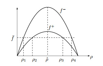
Flux functions
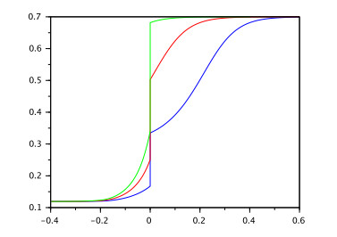
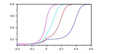
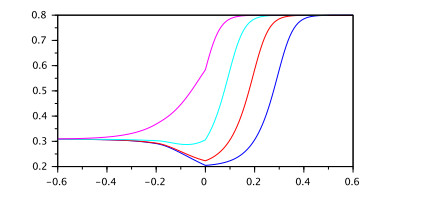
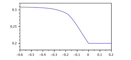
Sample traveling waves for Case A1, with
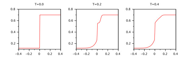
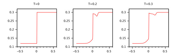
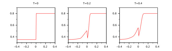
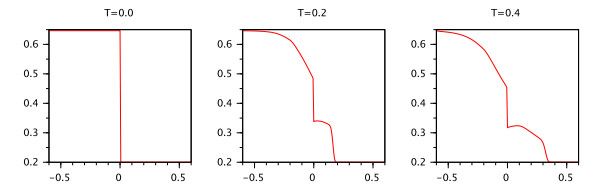
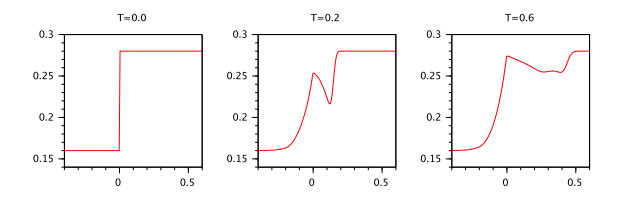
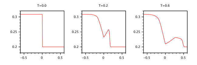
Numerical simulation for model (M1) with Riemann initial data for Case A1
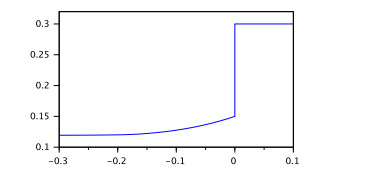
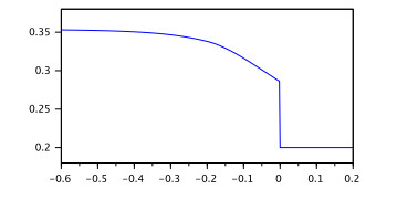
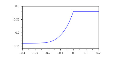
Typical traveling wave profile for Case A2
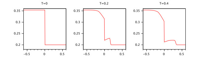
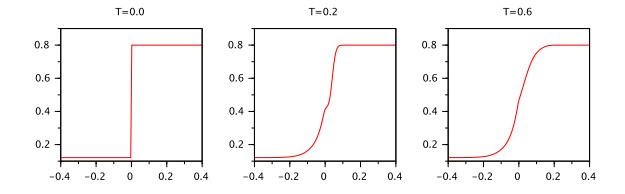
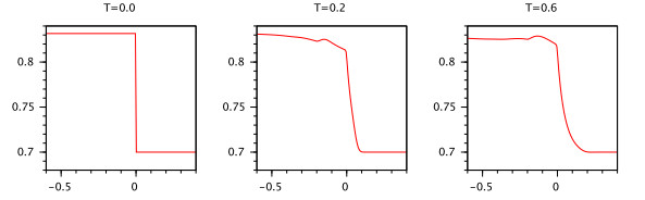
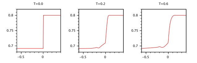
Numerical simulation for the PDE model with Riemann initial data for Case A2
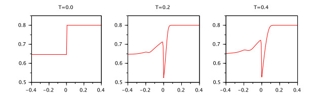
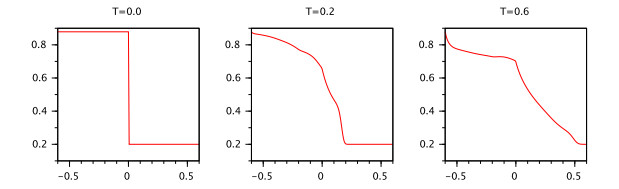
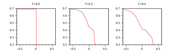
Numerical simulation for the PDE model with Riemann initial data for Case A3
Numerical simulation for the PDE model with Riemann initial data for Case A4
Sample traveling waves for Case B1
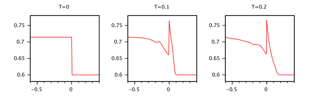
Numerical simulation for the PDE model with Riemann initial data for Case B1
Sample traveling wave for Case B2
Numerical simulation for the PDE model with Riemann initial data for Case B2
Numerical simulation for the PDE model with Riemann initial data for Case B3
Numerical simulation for the PDE model with Riemann initial data for Case B4
Sample traveling wave for Case C1
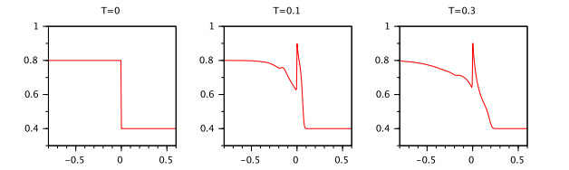
Numerical simulation for the PDE model with Riemann initial data for Case C1
Sample traveling wave for Case C2
Numerical simulation for the PDE model with Riemann initial data for Case C2
Numerical simulation for the PDE model with Riemann initial data for Case C3
Numerical simulation for the PDE model with Riemann initial data for Case C4
Sample traveling wave for Case D1
Numerical simulation for the PDE model with Riemann initial data for Case D1
Sample traveling wave for Case D2
Solution of Riemann problem for Case D2
Solution of Riemann problem for Case D3
Solution of Riemann problem for Case D4


 DownLoad: