We consider the general networks of elastic strings with Neumann boundary feedbacks and collocated observations in this paper. By selecting an appropriate multiplier, we show that this system is input-output $ L^2 $-well-posed. Moreover, we verify its regularity by calculating the input-output transfer function of system. In the end, by choosing an appropriate multiplier, we give a method to construct a Lyapunov functional and prove the exponential decay of tree-shaped networks with one fixed root under velocity feedbacks acted on all leaf vertices.
Citation: Dongyi Liu, Genqi Xu. Input-output $ L^2 $-well-posedness, regularity and Lyapunov stability of string equations on networks[J]. Networks and Heterogeneous Media, 2022, 17(4): 519-545. doi: 10.3934/nhm.2022007
We consider the general networks of elastic strings with Neumann boundary feedbacks and collocated observations in this paper. By selecting an appropriate multiplier, we show that this system is input-output $ L^2 $-well-posed. Moreover, we verify its regularity by calculating the input-output transfer function of system. In the end, by choosing an appropriate multiplier, we give a method to construct a Lyapunov functional and prove the exponential decay of tree-shaped networks with one fixed root under velocity feedbacks acted on all leaf vertices.

| [1] |
Remark on stabilization of tree-shaped networks of strings. Applications of Mathematics (2007) 52: 327-343. 
|
| [2] |
Stabilization of generic trees of strings. Journal of Dynamical and Control Systems (2005) 11: 177-193.
|
| [3] |
J. A. Bondy and U. S. R. Murty, Graph Theory, Springer-Verlag, New York, 2008. |
| [4] |
Regular linear systems governed by a boundary controlled heat equation. Journal of Dynamical and Control Systems (2002) 8: 341-370.
|
| [5] |
Well-posedness and regularity of Naghdi's shell equation under boundary control and observation. Journal of Differential Equations (2010) 249: 3174-3214.
|
| [6] |
Well-posedness of boundary control systems. SIAM Journal on Control and Optimization (2003) 42: 1244-1265.
|
| [7] |
The Salamon-Weiss class of well-posed infinite-dimensional linear systems: A survey. IMA Journal of Mathematical Control and Information (1997) 14: 207-223.
|
| [8] |
R. Dáger and E. Zuazua, Wave Propagation, Observation and Control in 1–d Flexible Multistructures, Springer Verlag, Berlin Heidelberg, 2006. |
| [9] |
R. Diestel, Graph Theory, 3$^{nd}$ edition, Springer-Verlag, Heidelberg, New York, 2005. |
| [10] |
Regularity of an Euler-Bernoulli equation with Neumann control and collocated observation. Journal of Dynamical and Control Systems (2006) 12: 405-418.
|
| [11] |
Well-posedness of systems of linear elasticity with dirichlet boundary control and observation. SIAM Journal on Control and Optimization (2009) 48: 2139-2167.
|
| [12] |
Variational and semigroup methods for waves and diffusion in networks. Applied Mathematics and Optimization (2007) 55: 219-240.
|
| [13] |
J. Lagnese, G. Leugering and E. J. P. G. Schmidt, Modeling, Analysis and Control of Dynamic Elastic Multi-link Structures, Systems and Control: Foundations and Applications, Birkhäuser, Inc., Boston, MA, 1994. |
| [14] |
$L_2(\Sigma)$-Regularity of the boundary to boundary operator $B^*L$ for hyperbolic and Petrowski PDEs. Abstract and Applied Analysis (2003) 19: 1061-1139.
|
| [15] | Riesz basis and stability properties for the feedback controlled networks of 1-D wave equations. WSEAS Transactions on Mathematics (2012) 11: 434-455. |
| [16] |
Stabilization of one-dimensional wave equations coupled with an ODE system on general tree-shaped networks. IMA Journal of Mathematical Control and Information (2015) 32: 557-589.
|
| [17] |
R. Mennicken and M. Moller, Non-self-adjoint Boundary Eigenvalue Problem, North-Holland mathematics studies 192, Elsevier, 2003. |
| [18] |
K. A. Morris, The well-posedness of accelerometer control systems,, in Analysis and Optimization of Systems: State and Frequency Domain Approaches for Infinite-Dimensional Systems (eds. R. F. Curtain, A. Bensoussan and J. L. Lions), Springer, Berlin, Heidelberg, 185 (1993), 378–387. |
| [19] |
M. A. Naimark, Linear Differential Operators (Part 1), Frederick Ungar, New York, 1967. |
| [20] |
Infinite dimensional linear systems with unbounded control and observation: A functional analytic approach. Transactions of the American Mathematical Society (1987) 300: 383-431.
|
| [21] |
Realization theory in Hilbert space. Mathematical Systems Theory (1989) 21: 147-164.
|
| [22] |
Super-stability and the spectrum of one-dimensional wave equations on general feedback controlled networks. IMA Journal of Mathematical Control and Information (2014) 31: 73-99.
|
| [23] |
(2005) Well-Posed Linear Systems. UK: Cambridge University Press.
|
| [24] |
Stabilization of the wave equation on 1-d networks. SIAM Journal on Control and Optimization (2009) 48: 2771-2797.
|
| [25] |
A characteristic equation associated to an eigenvalue problem on $c^2$-networks. Linear Algebra and Its Applications (1985) 71: 309-325.
|
| [26] |
Transfer functions of regular linear systems. Part Ⅰ: Characterizations of regularity. Transactions of the American Mathematical Society (1994) 342: 827-854.
|
| [27] |
The exponential decay rate of generic tree of 1-d wave equations with boundary feedback controls. Networks and Heterogeneous Media (2016) 11: 527-543.
|
| [28] |
Abstract second order hyperbolic system and applications to controlled networks of strings. SIAM Journal on Control and Optimization (2008) 47: 1762-1784.
|
| [29] |
Stability and spectral properties of general tree-shaped wave networks with variable coefficients. Acta Applicandae Mathematicae (2019) 164: 219-249.
|
| [30] |
Well-posedness and regularity of hyperbolic boundary control systems on a one-dimensional spatial domain. ESAIM: Control, Optimisation and Calculus of Variations (2010) 16: 1077-1093.
|

Figures(2) / Tables(2)
Dongyi Liu, Genqi Xu. Input-output $ L^2 $-well-posedness, regularity and Lyapunov stability of string equations on networks[J]. Networks and Heterogeneous Media, 2022, 17(4): 519-545. doi: 10.3934/nhm.2022007

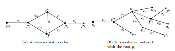
Networks consisting of strings with one fixed vertex
The tree-shaped network consisting of six strings with the fixed root


 DownLoad: