Loading [MathJax]/jax/output/SVG/jax.js

Nonlocal reaction traffic flow model with on-off ramps

  • Received: 01 August 2021 Revised: 01 December 2021 Published: 18 February 2022
  • Primary: 65M08; Secondary: 35L45, 90B20

  • We present a non-local version of a scalar balance law modeling traffic flow with on-ramps and off-ramps. The source term is used to describe the inflow and output flow over the on-ramp and off-ramps respectively. We approximate the problem using an upwind-type numerical scheme and we provide L and BV estimates for the sequence of approximate solutions. Together with a discrete entropy inequality, we also show the well-posedness of the considered class of scalar balance laws. Some numerical simulations illustrate the behaviour of solutions in sample cases.

    Citation: Felisia Angela Chiarello, Harold Deivi Contreras, Luis Miguel Villada. Nonlocal reaction traffic flow model with on-off ramps[J]. Networks and Heterogeneous Media, 2022, 17(2): 203-226. doi: 10.3934/nhm.2022003

    Related Papers:

    [1] Helge Holden, Nils Henrik Risebro . Follow-the-Leader models can be viewed as a numerical approximation to the Lighthill-Whitham-Richards model for traffic flow. Networks and Heterogeneous Media, 2018, 13(3): 409-421. doi: 10.3934/nhm.2018018
    [2] Michael Herty, J.-P. Lebacque, S. Moutari . A novel model for intersections of vehicular traffic flow. Networks and Heterogeneous Media, 2009, 4(4): 813-826. doi: 10.3934/nhm.2009.4.813
    [3] Paola Goatin, Sheila Scialanga . Well-posedness and finite volume approximations of the LWR traffic flow model with non-local velocity. Networks and Heterogeneous Media, 2016, 11(1): 107-121. doi: 10.3934/nhm.2016.11.107
    [4] Paola Goatin, Elena Rossi . Comparative study of macroscopic traffic flow models at road junctions. Networks and Heterogeneous Media, 2020, 15(2): 261-279. doi: 10.3934/nhm.2020012
    [5] Mauro Garavello . A review of conservation laws on networks. Networks and Heterogeneous Media, 2010, 5(3): 565-581. doi: 10.3934/nhm.2010.5.565
    [6] Ye Sun, Daniel B. Work . Error bounds for Kalman filters on traffic networks. Networks and Heterogeneous Media, 2018, 13(2): 261-295. doi: 10.3934/nhm.2018012
    [7] Edward S. Canepa, Alexandre M. Bayen, Christian G. Claudel . Spoofing cyber attack detection in probe-based traffic monitoring systems using mixed integer linear programming. Networks and Heterogeneous Media, 2013, 8(3): 783-802. doi: 10.3934/nhm.2013.8.783
    [8] Simone Göttlich, Ute Ziegler, Michael Herty . Numerical discretization of Hamilton--Jacobi equations on networks. Networks and Heterogeneous Media, 2013, 8(3): 685-705. doi: 10.3934/nhm.2013.8.685
    [9] Abraham Sylla . Influence of a slow moving vehicle on traffic: Well-posedness and approximation for a mildly nonlocal model. Networks and Heterogeneous Media, 2021, 16(2): 221-256. doi: 10.3934/nhm.2021005
    [10] Michael Herty, Lorenzo Pareschi, Mohammed Seaïd . Enskog-like discrete velocity models for vehicular traffic flow. Networks and Heterogeneous Media, 2007, 2(3): 481-496. doi: 10.3934/nhm.2007.2.481
  • We present a non-local version of a scalar balance law modeling traffic flow with on-ramps and off-ramps. The source term is used to describe the inflow and output flow over the on-ramp and off-ramps respectively. We approximate the problem using an upwind-type numerical scheme and we provide L and BV estimates for the sequence of approximate solutions. Together with a discrete entropy inequality, we also show the well-posedness of the considered class of scalar balance laws. Some numerical simulations illustrate the behaviour of solutions in sample cases.


    Models of conservation laws with nonlocal flux have been used to describe traffic flow dynamics in which drivers adapt their velocity with respect to what happens to the cars in front of them [3,5,9,11,18]. In this type of models, the flux function depends on a downstream convolution term between the density or the velocity of vehicles and a kernel function with support on the negative axis. However, the above models cannot be used to study the traffic flow on the highway with ramps since they did not include their presence. Indeed, ramps are an important element of traffic systems and develop some complex traffic phenomena, see [12,15,16,19,20,21,22].

    In this work, we propose a new nonlocal traffic model which includes the effects of the inflow and output flow over the on- and off- ramps respectively. We start by considering a modified local reaction traffic model proposed in [16],

    ρt+(ρv(ρ))x=SonSoff, (1.1)

    where the non-negative functions Son and Soff are the source and sink term, respectively, defined by

    Son(t,x,ρ)=1on(x)qon(t)(1ρρmax), (1.2)
    Soff(t,x,ρ)=1off(x)qoff(t)ρρmax, (1.3)

    where qonR+, and qoffR+ the rate (number of vehicles per unit time per unit length) of the on- and off-ramp respectively, as in [20,21],

    qon(t)=qrampon(t)Lon,qoff(t)=qrampoff(t)Loff,

    with qrampon(t) the expected inflow flow of the on-ramp and qrampoff(t) the expected output flow of the off-ramp, Lon and Loff are the lengths of the on- and off-ramps respectively, whose spatial positions are described by the indicator functions 1on(x) and 1off(x), defined as

    1on(x)={1xΩon:=[x_on,¯xon],0otherwise,1off(x)={1xΩoff:=[x_off,¯xoff],0otherwise.

    For simplicity we consider Lon=Loff=L in the whole paper.

    In order to obtain a non-local version of the model (1.1), we first rewrite the flux function f(ρ)=ρv(ρ) in its non-local version, where drivers react adapting their velocity with respect to what happens in front of them, see [1,3,5,11],

    f(ρ)=ρv(ρωη),with(ρωη)(t,x)=x+ηxρ(t,y)ωη(yx)dy.

    On the on-ramp the idea is that at position x the flow merging in the traffic way is inversely proportional to the average density around position x+δ, see Fig. 1, i.e, we write

    Son(t,x,ρ,ρωη,δ)=1on(x)qon(t)(1ρωη,δρmax), (1.4)
    Figure 1. 

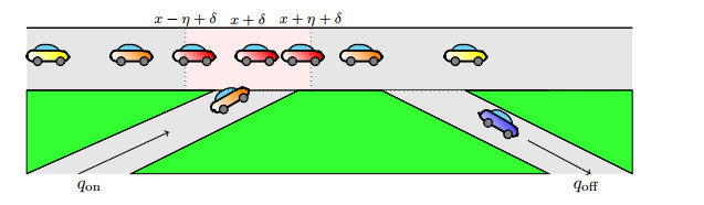
    Illustration of the model setting

    .

    where

    (ρωη,δ)(t,x)=x+η+δxη+δρ(t,y)ωη,δ(yx)dy,

    with η[0,1] and δ[η,η]. {Similarly to [5], here the parameter η represents the radius of the support of the kernel function ωη,δ, while δ is the point at which the maximum is attained. This choice of the kernel models the fact that drivers on the on-ramp can see what happens on the backward and forward on the main road.} However, in the numerical test section we will see that the choice of the non-local term (1.4) does not guarantee that the proposed model satisfies a Maximum Principle, see Example 3. In order to overcome this difficulty, we consider a first variant of (1.4) taking

    Son(t,x,ρ,ρωη,δ)=1on(x)qon(t)(1ρρmax)(1ρωη,δρmax). (1.5)

    Note that this term contains a product which differentiates it from the original model, this choice is also assumed in the multilane model studied in [8]. An alternative to avoid the double product in the previous equation (1.5) is the following

    Son(t,x,ρ,ρωη,δ)=1on(x)qon(t)(1max{ρρmax;ρωη,δρmax}). (1.6)

    {In both models with (1.5) and (1.6), if the main road is crowded only few vehicles can enter to the main road.}

    The purpose of this work is the study of the well-posedness of a nonlocal reaction traffic flow model with source term given by (1.5) and (1.6).

    In [2,3,4,5,6,9,11] the authors studied a nonlocal conservation law to model vehicular traffic flow in the case Son=Soff=0, i.e., without on- and off-ramps. The need to design more realistic models has led to the development of multi-lane vehicular traffic models among which we can highlight the following. In [14] it is introduced a new local model for multilane dense vehicular traffic by means of a system of a weakly coupled scalar conservation laws. In [10] the authors consider the model proposed in [14] but with a more general source term and they allow for the presence of space discontinuities both in the speed law and in the number of lanes; in these two local models the source term accounts for the lane change rate and the key assumption is that the drivers prefer to drive faster, and that the tendency of a vehicle to change lanes is proportional to the difference in velocity between neighboring lanes. In [8] a multilane model with local and non-local flux combined with a source term that also incorporates a nonlocality is studied; here, the non-local source term describes the lane changing rate depending on a (nonlinear) evaluation of the velocity. In particular, the lane changing rate is proportional to the difference in the velocity between two adjacent lanes, but the velocities are evaluated in a neighbourhood of the current position, moreover, this rate is proportional also to the density in the receiving lane, meaning that if that lane is crowded only a few vehicles can actually change lane.

    Regarding to vehicular traffic flow models taking into account the presence of ramps, we can mention [16], where the authors study the (local) first order nonlinear conservation law (1.1). A (local) second order model is proposed in [21] to study the effects of on- and off-ramps on a main road during two rush periods. Likewise, other works about the study of effects of ramps in vehicular traffic flow models are referenced in [21]. In particular, in [7] the authors consider a Lighthill-Witham-Richards (LWR) traffic flow model on a junction composed by one mainline, an on-ramp and an off-ramp, which are connected by a node. Moreover, in [13] a non-local gas-kinetic traffic model including ramps is proposed, the model allows to simulate syncronized congested traffic and reproduces realistic phenomena of vehicular traffic by variations of the on-ramp flow. A new modeling methodology for merging and diverging flows is studied in [17], the methodology includes coupling effects between main and ramps flows and a new formulation for the modeling of traffic friction is also introduced.

    This work is organized as follows. In Section 2 we present the proposed mathematical model with all the considered assumptions on it. Afterwards, we introduce an upwind-type scheme with two different source terms and derive important properties such as maximum principle, L1 bound and BV estimates. Furthermore, we derive the L1Lipschitz continuous dependence of solutions to (2.1) on the initial data and the terms qon and qoff in Section 3. In Section 4, we present numerical examples illustrating the behavior of the solutions of our model.

    The main goal of this work is to study the well-posedness of the non-local reaction traffic model

    ρt+(ρv(ρωη))x=Son(,,ρ,ρωη,δ)Soff(,,ρ),xR, (2.1)

    where Son(,,ρ,ρωη,δ) defined in (1.5) or (1.6), Soff defined by (1.3) and initial condition

    ρ(x,0)=ρ0(x)(L1BV)(R,[0,ρmax]). (2.2)

    From now on we call Model 0 the equations (2.1)-(1.4)-(2.2), Model 1 the equations (2.1)-(1.5)-(2.2), and Model 2 (2.1)-(1.6)-(2.2). Let us assume the following assumptions:

    qramponL(R+;R+),qrampoffL(R+;R+).vC2([0,ρmax];R+), v(ρ)0,ρ[0,ρmax].ωηC1([0,η];R+) with ωη(x)0, η0ωη(x)dx=1, η>0.ωη,δC1([δη,δ+η];R+) with ω(x)η,δ0 for x[δη,0],ω(x)η,δ0  for x[0,δ+η], and δ+ηδηωη,δ(x)dx=1, η>0. (H1)

    We recall the definition of weak entropy solution for (2.1).

    Definition 2.1. Let ρ0(L1BV)(R;[0,ρmax]). We say that ρC([0,T];L1(R;[0,ρmax])), with ρ(t,)BV(R;[0,ρmax]) for t[0,T], is a weak solution to (2.1) with initial datum ρ0 if for any φC1c([0,T[×R;R)

    T0R(ρφt+ρVφx)dxdt+T0ΩonSonφdxdtT0ΩoffSoffφdxdt+Rρ0(x)φ(0,x)dx=0,

    where V(t,x)=v((ρω)(t,x)) and Son is as in (1.5) or (1.6).

    Definition 2.2. Let ρ0(L1BV)(R;[0,ρmax]). We say that ρC([0,T];L1(R;[0,ρmax])), with ρ(t,)BV(R;[0,ρmax]) for t[0,T], is a entropy weak solution to (2.1) with initial datum ρ0 if for any φC1c([0,T[×R;R) and for all kR

    T0R(|ρk|φt+|ρk|Vφxsgn(ρk)kVxφ)dxdt+T0Ωonsgn(ρk)SonφdxdtT0Ωoffsgn(ρk)Soffφdxdt+R|ρ0k|φ(0,x)dx0.

    Our main result is given by the following theorem, which states the well-posedness of problem (2.1) to (2.2) with source term given by (1.5) or (1.6). In order to simplify the computations we consider ρmax=1 from now on.

    Theorem 2.1. Let ρ0(L1BV)(R;[0,1]). Assume vC2([0,1];R+). Then, for all T>0, the problem (2.1) has a unique solution ρC0([0,T];L1(R;[0,1])) in the sense of Definition 2.2. Moreover, the following estimates hold: for any t[0,T]

    ρ(t)L1(R)R1(t),0ρ(t,x)1,TV(ρ(t))etH(TV(ρ0)+tQT),

    where

     R1=ρ0L1(R)+qrampon()L1([0,t])minxΩonqrampon()ρ(,x)L1([0,t])minxΩoffqrampoff()ρ(,x)L1([0,t]), (2.3)
    QT=2(qonL([0,T])+qoffL([0,T])), (2.4)
    H=2qonL([0,T])+qoffL([0,T])+ωη(0)L, (2.5)
    L=(vL([0,1])+vL([0,1])). (2.6)

    We take a space step Δx such that η=NΔx, for some NN, and a time step Δt subject to a CFL condition which will be specified later. For any jZ, let xj1/2=jΔx be a cells interfaces, xj=(j+12)Δx the cells centers. We consider ramps with length L and take L=Δx, for some Z+ such that x_on=xk_on+1/2, ¯xon=xk_on+1/2+, x_off=xk_off+1/2 and ¯xoff=xk_off+1/2+, for some k_on,k_offZ. With this notation, we define the subdomains Ωon=[x_on,¯xon], Ωoff=[x_off,¯xoff], and we put Ωkon=[k_on+1,k_on+] and Ωkoff=[k_off+1,k_off+]. We fix T>0, and set NTN such that NTΔtT<(NT+1)Δt and define the time mesh as tn=nΔt for n=0,,NT. Set λ=Δt/Δx. The initial data is approximated for jZ, as follows:

    ρ0j=1Δxxj+1/2xj1/2ρ0(x)dx.

    We define a piecewise constant approximate solution ρΔ(t,x) to (2.1) as

    ρΔ(t,x)=ρnj, for {t[tn,tn+1[x]xj1/2,xj+1/2],where n=0,,NT1,jZ. (3.1)

    The Son terms (1.5) and (1.6) are discretized via

    Son(tn+1/2,xj,ρn+1/2j,Rn+1/2on,j)=1on,jqn+1/2on(1ρn+1/2j)(1Rn+1/2on,j), (3.2)
    Son(tn+1/2,xj,ρn+1/2j,Rn+1/2on,j)=1on,jqn+1/2on(1max{ρn+1/2j,Rn+1/2on,j}). (3.3)

    The Soff term is discretizated via

    Soff(tn+1/2,xj,ρn+1/2j)=1off,jqn+1/2offρn+1/2j, (3.4)

    where we denote

    1on,j={1Δxxj+1/2xj1/21on(x)dx,x_onxj¯xon,0otherwise.
    1off,j={1Δxxj+1/2xj1/21off(x)dx,x_offxj¯xoff,0otherwise.
    qn+1/2on=1Δttn+1tnqon(t)dt,qn+1/2off=1Δttn+1tnqoff(t)dt.

    The approximate solution ρΔ is obtained via an upwind-type scheme together with operator splitting to account for the reaction term, see Algorithm 3.1.

    Algorithm 3.1 (Upwind scheme).

    Input: approximate solution vector {ρnj}jZ for t=tn

    do jZ

    ρn+1/2jρnjλ(ρnjv(Rnj+1/2)ρnj1v(Rnj1/2)) (3.5)

    enddo

    do jZ

    Sn+1/2on,jSon(tn+1/2,xj,ρn+1/2j,Rn+1/2on,j), using (3.2) or (3.3),

    Sn+1/2off,jSoff(tn+1/2,xj,ρn+1/2j), using (3.4),

    ρn+1jρn+1/2j+ΔtSn+1/2on,jΔtSn+1/2off,j (3.6)

    enddo

    Output: approximate solution vector {ρn+1j}jZ for t=tn+1=tn+Δt.

    The terms Rnj+1/2, Rn+1/2on,j for jZ and n=0,,NT1 denotes the discrete convolution operators in the velocity and source term and they are defined, respectively, by

    Rnj+1/2=η/Δx1p=0γpρnj+p+1,Rn+1/2on,j=δ+ηΔx1h=δηΔxˆγhρn+1/2j+h.

    Here we denote γp=xp+1/2xp1/2ωη(yx)dy, for p[0,η/Δx1] and ˆγh=xh+1/2xh1/2ωη,δ(yx)dy, for h[(δη)/Δx,(δ+η)/Δx1].

    Remark 3.1. If 0ρn+1/2j1 for all jZ, then for all n{0,,NT1},

    Rn+1/2onL(Ωkon)1. Indeed, we have that

    |Rn+1/2on,j|δ+ηΔx1h=δηΔxˆγh|ρn+1/2j+h+1|δ+ηΔx1h=δηΔxˆγh=1.

    Remark 3.2. The discrete convolution operator Rn+1/2on,j satisfies

    jZ|Rn+1/2on,j+1Rn+1/2on,j|jZ|ρn+1/2j+1ρn+1/2j|.

    The proof of this property can be seen in [8] Lemma 3.2.

    In order to prove the existence of solution of model (2.1)-(1.5), in the next lemmas we will show some properties of the approximate solutions constructed by the Algorithm 3.1.

    Lemma 3.1 (Maximum principle). Let ρ0L(R;[0,1]). Let hypotheses (H1) and the following Courant-Friedrichs-Levy (CFL) condition hold

    Δtmin{Δx(γ0vL([0,1])+vL([0,1])),1QT}, (3.7)

    with QT defined in (2.4) then for all t>0 and xR the piece-wise constant approximate solution ρΔ constructed through Algorithm 3.1 is such that

    0ρΔ(t,x)1.

    Proof. The proof is made by induction. Let us assume that 0ρnj1 for all jZ. Consider the convective step (3.5) of Algorithm 3.1, by CFL condition (3.7) we have 0ρn+1/2j1 for jZ (see Theorem 3.3 of [9]).

    Now focus on the remaining step, involving the source term.

    ρn+1j=ρn+1/2j+Δt(1on,jqn+1/2on(1ρn+1/2j)(1Rn+1/2on,j)1off,jqn+1/2offρn+1/2j)ρn+1/2j+Δt1on,jqn+1/2on(1ρn+1/2j)Δt1off,jqn+1/2offρn+1/2j=(1Δt(1on,jqn+1/2on+1off,jqn+1/2off))ρn+1/2j+Δt1on,jqn+1/2on.

    Because of CFL condition (3.7), the last right-hand side is a convex combination of ρn+1/2j and one. Then ρn+1j[ρn+1/2j,1] and since ρn+1/2j[0,1], we therefore conclude that 0ρn+1j1, for jZ.

    Lemma 3.2 (L1Bound). Let ρ0L1(R,[0,1]). Let (H1) and the CFL condition (3.7) hold. Then, the piece-wise constant approximate solution ρΔ constructed through Algorithm 3.1 satisfies, for all T>0,

    ρΔ(T,)L1(R)C1(T),

    with

    C1(t)=ρ0L1(R)+qramponL1([0,t])minxΩonqrampon()ρΔ(,x)L1([0,t])minxΩoffqrampoff()ρΔ(,x)L1([0,t]). (3.8)

    Proof. For the conservative form of the scheme (3.5), it is satisfied

    ρn+1/2L1(R)=ρnL1(R).

    Now, we going to work L1 norm for relaxation step (3.6). By Remark 3.1 and CFL condition (3.7) we have

    |ρn+1j||ρn+1/2j|+Δt1on,jqn+1/2on(1|ρn+1/2j|)Δt1off,jqn+1/2off|ρn+1/2j|, (3.9)

    multiplying this inequality by Δx and summing over all jZ we obtain

    ρn+1L1(R)ρn+1/2L1(R)+Δtqn+1/2onΔx(jΩkon1on,jjΩkon1on,j|ρn+1/2j|)Δtqn+1/2offΔxjΩkoff1off,j|ρn+1/2j|ρnL1(R)+ΔtLqn+1/2on(1minjΩkonρn+1/2j)ΔtLqn+1/2offminjΩkoffρn+1/2j=ρnL1(R)+ΔtLqn+1/2onΔtminjΩkonLqn+1/2onρn+1/2jΔtminjΩkoffLqn+1/2offρn+1/2j.

    Thus, by a standard iterative procedure we can deduce

    ρnL1(R)ρ0L1(R)+qramponL1([0,T])minxΩonqrampon()ρΔ(,x)L1([0,T])minxΩoffqrampoff()ρΔ(,x)L1([0,T]).

    We first prove the Lipschitz continuity of the source terms (3.2) in its second, third and fourth argument and of (3.4) in its second and third argument.

    Lemma 3.3. The map Son defined in (3.2) is Lipschitz continuous in second, third and fourth argument with Lipschitz constant qonL([0,T]), and the map Soff defined in (3.4) is Lipschitz continuous in second and third argument with Lipschitz constant qoffL([0,T]).

    Proof. Let us start with term (3.2). We denote

    Son=Son(t,x,ρ,Ron)Son(t,˜x,˜ρ,˜Ron),

    then

    |Son||Son(t,x,ρ,Ron)Son(t,x,˜ρ,Ron)|+|Son(t,x,˜ρ,Ron)Son(t,x,˜ρ,˜Ron)|+|Son(t,x,˜ρ,˜Ron)Son(t,˜x,˜ρ,˜Ron)|=|1onqon(1Ron)(˜ρρ)|+|1onqon(1˜ρ)(˜RonRon)|+|(1on˜1on)qon(1˜ρ)(1˜Ron)|qonL([0,T])|˜ρρ|+qonL([0,T])|˜RonRon|+qonL([0,T])|1on˜1on|qonL([0,T])(|˜ρρ|+|˜RonRon|+|1on˜1on|).

    Now, we prove the Lipschitz continuity of Soff term (3.4). Denoting

    Soff=Soff(t,x,ρ)Soff(t,˜x,qoff,˜ρ), we get

    |Soff||Soff(t,x,ρ)Soff(t,˜x,ρ,)|+|Soff(t,˜x,ρ)Soff(t,˜x,˜ρ)|=|1offqoffρ˜1offqoffρ|+|˜1offqoffρ˜1offqoff˜ρ|qoffL([0,T])(|1off˜1off|+|ρ˜ρ|),

    Thus, we have completed the proof.

    The Lipschitz continuity of the source term proved in Lemma 3.3 is one of the key ingredients in order to prove the following total variation bound on the numerical approximation.

    Proposition 3.1 (BV estimate in space). Let ρ0(L1BV)(R;[0,1]). Assume that the hypotheses (H1) and CFL condition (3.7) hold. Then, for n=0,,NT1 the following estimate holds

    jZ|ρnj+1ρnj|eTH(TV(ρ0)+TQT),

    with QT like in (2.4) and H like in (2.5).

    Proof. Let us compute

    ρn+1j+1ρn+1j=ρn+1/2j+1ρn+1/2j+Δt[Sn+1/2on,j+1Sn+1/2on,j]Δt[Sn+1/2off,j+1Sn+1/2off,j].

    By the Lipschitz continuity of the source term proved in Lemma 3.3 and the property of the discrete convolution operator given in Remark 3.2, we get

    jZ|ρn+1j+1ρn+1j|(1+ΔtqonL([0,T]))jZ|ρn+1/2j+1ρn+1/2j|+ΔtqonL([0,T])jΩkon|1on,j+11on,j|+ΔtqonL([0,T])jZ|Rn+1/2on,j+1Rn+1/2on,j|+ΔtqoffL([0,T])jZ|ρn+1/2j+1ρn+1/2j|+ΔtqoffL([0,T])jΩoff|1off,j+11off,j|(1+Δt(2qonL([0,T])+qoffL([0,T])))jZ|ρn+1/2j+1ρn+1/2j|+ΔtqonL([0,T])jΩkon|1on,j+11on,j|+ΔtqoffL([0,T])jΩoff|1off,j+11off,j|(1+Δt(2qonL([0,T])+qoffL([0,T])))jZ|ρn+1/2j+1ρn+1/2j|+ΔtQT. (3.10)

    Now, for convective part (3.5) we follow [9] and get

    |ρn+1/2j+1ρn+1/2j|(1+Δtωη(0)L)jZ|ρnj+1ρnj|,

    with L=(vL([0,1])+vL([0,1])). Plugging the inequality above in (3.10) we obtain

    jZ|ρn+1j+1ρn+1j|(1+Δt(2qonL([0,T])+qoffL([0,T])))×(1+Δtωη(0)L)jZ|ρnj+1ρnj|+ΔtQT,

    which applied recursively yields

    jZ|ρnj+1ρnj|eTH(TV(ρ0)+TQT), (3.11)

    with H=2qonL([0,T])+qoffL([0,T])+ωη(0)L.

    Proposition 3.2 (BV estimate in space and time). Let hypotheses (H1) hold, ρ0(L1BV)(R;[0,1]). If the CFL condition (3.7) holds, then, for every T>0 the following discrete space and time total variation estimate is satisfied:

    TV(ρΔ;[0,T]×R)TCxt(T),

    with

    Cxt(T)=eTH((1+2L)(TV(ρ0)+TQT))+12QTC1(T)+qramponL([0,T]). (3.12)

    Proof.

    TV(ρΔ;[0,T]×R)=NT1n=0jZΔt|ρnj+1ρnj|+(TNTΔt)jZ|ρNTj+1ρNTj|+NT1n=0jZΔx|ρn+1jρnj|.

    By BV estimate in space (3.11), we have

    NT1n=0jZΔt|ρnj+1ρnj|+(TNTΔt)jZ|ρNTj+1ρNTj|TeTH(TV(ρ0)+TQT). (3.13)

    On the other hand, observe that

    |ρn+1jρnj||ρn+1jρn+1/2j|+|ρn+1/2jρnj|. (3.14)

    We then estimate separately each term on the right hand side of the inequality (3.14).

    By the definition of the relaxation step (3.6), for the first term on right hand side of (3.14) we have

    |ρn+1jρn+1/2j|Δt|Sn+1/2on,jSn+1/2off,j|Δt1on,jqn+1/2on(1ρn+1/2j)(1Rn+1/2on,j)+Δt1off,jqn+1/2offρn+1/2jΔtqn+1/2on(1on,j+1on,j|ρn+1/2j|)+Δt1off,jqn+1/2off|ρn+1/2j|, (3.15)

    then multiplying by Δx and summing over all jZ,

    ΔxjZ|ρn+1jρn+1/2j|Δtqn+1/2on(ΔxjΩkon1on,j+ΔxjΩkon1on,j|ρn+1/2j|)+Δtqn+1/2offΔxjΩkoff1off,j|ρn+1/2j|Δtqn+1/2on(L+ρn+1/2L1(R))+Δtqn+1/2offρn+1/2L1(R)=Δtqn+1/2on(L+ρnL1(R))+ΔtqoffL([0,T])ρnL1(R)=12ΔtQTρnL1(R)+ΔtqramponL([0,T]). (3.16)

    Now we analyze the second term of the right hand side (3.14). Since the numerical flux defined in (3.5) is Lipschitz continuous in both arguments with Lipschitz constant L, defined by (2.6), we obtain

    |ρn+1/2jρnj|=λ|Fj+1/2(ρnj,Rnj+1/2)Fj1/2(ρnj1,Rnj1/2)|λL(|ρnjρnj1|+|Rnj+1/2Rnj1/2|),

    multiplying by Δx, summing over all jZ and by the Remark 3.2 we get

    ΔxjZ|ρn+1/2jρnj|2LΔtjZ|ρnj+1ρnj|. (3.17)

    Collecting together (3.16) and (3.17), and by using Lemma 3.2 and Proposition 3.1 we have,

    ΔxjZ|ρn+1jρnj|12ΔtQTρnL1(R)+ΔtqramponL([0,T])+2LΔtjZ|ρnj+1ρnj|12ΔtQTC1(T)+ΔtqramponL([0,T])+2LΔteTH(TV(ρ0)+TQT). (3.18)

    Then, collecting together (3.13) and (3.18) we get

    NT1n=0jZΔt|ρnj+1ρnj|+(TNTΔt)jZ|ρNTj+1ρNTj|+NT1n=0jZΔx|ρn+1jρnj|TeTH((1+2L)(TV(ρ0)+TQT))+12TQTC1(T)+TqramponL([0,T]).

    In order to define an entropy inequality we define, for κ[0,1], and the numerical fluxes

    Gj+1/2(u)=uv(Rj+1/2),Fκj+1/2(u)=Gj+1/2(uκ)Gj+1/2(uκ),

    with ab=max{a,b}, and ab=min{a,b}.

    Lemma 3.4. Let ρ0(L1BV)(R;[0,1]). Assume that hypotheses (H1) and CFL condition (3.7) hold. Then, the approximate solution ρΔ constructed by Algorithm 3.1 satisfies the following discrete entropy inequality: for jZ, for n=0,,NT1 and for any κ[0,1],

    |ρn+1jκ||ρnjκ|+λ(Fkj+1/2(ρnj)Fkj+1/2(ρnj1))Δtsgn(ρn+1jκ)(Son(tn+1/2,xj,ρn+1/2j,Rn+1/2on,j)Soff(tn+1/2,xj,ρn+1/2j))+λsgn(ρn+1jκ)κ(v(Rnj+1/2)v(Rnj1/2))0.

    Proof. We set

    Gj(u,w)=wλ(Gj+1/2(w)Gj1/2(u))=wλ(wv(Rj+1/2)uv(Rj1/2)).

    Clearly ρn+1/2j=Gj(ρnj1,ρnj).

    The map Gj is a monotone non-decreasing function with respect to each variable under the CFL condition (3.7) since we have

    Gw=1λv(Rj+1/2)0,Gu=λv(Rj1/2).

    Moreover, we have the following identity

    Gj(ρnj1κ,ρnjκ)Gj(ρnj1 κ,ρnjκ)=|ρnjκ|λ(Fkj+1/2(ρnj)Fkj1/2(ρnj1)).

    Then, by monotonicity, the definition of scheme (3.5) and by using

    |a+b||a|+sgn(a)b, we get

    Gj(ρnj1κ,ρnjκ)Gj(ρnj1 κ,ρnjκ)Gj(ρnj1,ρnj)Gj(κ,κ)Gj(ρnj1,ρnj)Gj(κ,κ)=|Gj(ρnj1,ρnj)Gj(κ,κ)|=|ρn+1/2jGj(κ,κ)|=|ρn+1jκ+λκ(v(Rnj+1/2)v(Rnj1/2))Δt(Son(tn+1/2,xj,ρn+1/2j,Rn+1/2on,j)Soff(tn+1/2,xj,ρn+1/2j))||ρn+1jκ|+λsgn(ρn+1jκ)κ(v(Rnj+1/2)v(Rnj1/2))Δtsgn(ρn+1jκ)(Son(tn+1/2,xj,ρn+1/2j,Rn+1/2on,j)Soff(tn+1/2,xj,ρn+1/2j)).

    The following Theorem states the L1-Lipschitz continuous dependence of solution to (2.1) on both the initial datum and the qon and qoff functions.

    Theorem 3.1 (Uniqueness). Let ρ and ˜ρ be two solutions to problem (2.1) in the sense of Definition 2.2, with initial data ρ0, ˜ρ0L1BV(R;[0,1]), with on-ramp rate qon, ˜qon and off-ramp rate qoff, ˜qoff, respectively. Assume vC2([0,1],R+). Then, for a.e. t[0,T],

    ρ(t)˜ρ(t)L1(R)eCT(ρ0˜ρ0L1(R)+L(qon˜qonL1([0,t])+qoff˜qoffL1([0,T]))).

    Proof. The proof follows closely Theorem 5.6 of [8].

    By using Kružkov's doubling of variables technique we get

    ρ(T,)˜ρ(T,)L1(R)ρ0˜ρ0L1(R)+T0Ωon|˜Son|dxdt+T0Ωoff|˜Soff|dxdt+T0R|V||xρ(t,x)|dxdt+T0R|Vx||ρ(t,x)|dxdt,

    where

    ˜Son=Son(t,x,qon,ρ,Ron)Son(t,x,˜qon,˜ρ,˜Ron),˜Soff=Soff(t,x,qon,ρ)Soff(t,x,˜qon,˜ρ),V=v(R)v(P),Vx=xv(R)xv(P).

    Let us now estimate all the terms appearing in the right hand side of the above inequality. We start bounding ˜Son and ˜Soff terms:

    T0Ωon|˜Son|dxdt=T0Ωon|Son(t,x,qon,ρ,Ron)Son(t,x,˜qon,˜ρ,˜Ron)|dxdtT0Ωon(|˜S1on|+|˜S2on|+|˜S3on|)dxdt,

    where

    ˜S1on=Son(t,x,qon,ρ,Ron)Son(t,x,qon,ρ,˜Ron),˜S2on=Son(t,x,qon,ρ,˜Ron)Son(t,x,qon,˜ρ,˜Ron),˜S3on=Son(t,x,qon,˜ρ,˜Ron)Son(t,x,˜qon,˜ρ,˜Ron).

    First we are going to bound ˜S1on term,

    |˜S1on|=|1onqon(1ρ)((1Ron)(1˜Ron))|qonL([0,T])|˜RonRon|,

    thus

    T0Ωon|˜S1on|dxdtqonL([0,T])T0Ωon|˜RonRon|dxdtqonL([0,T])T0˜RonRonL1(Ωon).

    Observe that

    Ron˜RonL1(Ωon)ρ(t,)˜ρ(t,)L1(Ωon),

    since Rωη(x)dx=1. Then,

    T0Ωon|˜S1on|dxdtqonL([0,T])T0ρ(t,)˜ρ(t,)L1(Ωon)dtqonL([0,T])T0ρ(t,)˜ρ(t,)L1(R)dt.

    Now we are going to bound ˜S2on.

    |˜S2on|=|1onqon(1˜Ron)(1ρ)(˜ρρ)|qonL([0,T])|ρ˜ρ|.

    Integrating in time and space we have

    T0Ωon|˜S2on|dxdtqonL([0,T])T0ρ(t,)˜ρ(t,)L1(Ωon)dtqonL([0,T])T0ρ(t,)˜ρ(t,)L1(R)dt.

    Bounding ˜S3on,

    |˜S3on|=|1on(1˜ρ)(1˜Ron)(qon˜qon)||qon˜qon|,

    thus

    T0Ωon|˜S3on|dxdtT0Ωon|qon˜qon|dxdtLqon˜qonL1([0,T]).

    Therefore, we get the following estimate

    T0Ωon|˜Son|dxdt2qonL([0,T])T0ρ(t,)˜ρ(t,)L1(R)dt+Lqon˜qonL1([0,T]). (3.19)

    Regarding ˜Soff term, we proceed in a similar way like above and we get

    |˜Soff|=|1offqoffρ1off˜qoff˜ρ||˜S1off|+|˜S2off|,

    where

    ˜S1off=Soff(t,x,qoff,ρ)Soff(t,x,qoff,˜ρ),˜S2off=Soff(t,x,qoff,˜ρ)Soff(t,x,˜qoff,˜ρ).

    Then,

    T0Ωoff|˜S1off|dxdtqoffL([0,T])T0ρ(t,)˜ρ(t,)L1(Ωoff)dtqoffL([0,T])T0ρ(t,)˜ρ(t,)L1(R)dt,

    and

    T0Ωoff|˜S2off|dxdtLqoff˜qoffL1([0,T]).

    Thus, we get

    T0Ωoff|Soff|dxdtqoffL([0,T])T0ρ(t,)˜ρ(t,)L1(R)dt+Lqoff˜qoffL1([0,T]). (3.20)

    {Next, focus on V, by using the following estimate

    |V|ωη(0)vL([0,1])ρ(t,)˜ρ(t,)L1(R),

    we obtain}

    T0R|V||xρ(t,x)|dxdtωη(0)vL([0,1])supt[0,T]ρ(t,)TV(R)T0ρ(t,)˜ρ(t,)L1(R)dt. (3.21)

    Next, we pass to Vx. Following [8] we compute

    |Vx|(2(ωη(0))2v"L([0,1])+vL([0,1])ωηL([0,η]))ρ(t,)˜ρ(t,)L1(R)+ωη(0)vL([0,1])(|ρ˜ρ|(t,x+η)+|ρ˜ρ|(t,x)),

    thus

    T0R|Vx||ρ(t,x)|dxdtWT0ρ(t,)˜ρ(t,)L1(R)dt, (3.22)

    where

    W=(2(ωη(0))2v"L([0,1])+vL([0,1])ωηL([0,η]))C1(t)+2ωη(0)vL([0,1]).

    Collecting together (3.19), (3.20), (3.21) and (3.22) we get

    ρ(T,)˜ρ(T,)L1(R)ρ0˜ρ0L1(R)+L(qon˜qonL1([0,t])+qoff˜qoffL1([0,t]))+CT0ρ(t,)˜ρ(t,)L1(R)dt, (3.23)

    where

    C=H+ωη(0)vL([0,1])supt[0,T]ρ(t,)TV(R)+W. (3.24)

    An application of Gronwall Lemma to (3.23) completes the proof.

    The convergence of the approximate solutions constructed by Algorithm 3.1 towards the unique weak entropy solution can be proven by applying Helly's compactness theorem. The latter can be applied due to Lemma 3.1 and Proposition 3.2 and states that there exists a sub-sequence of approximate solution ρΔ that converges in L1 to a function ρL([0,T]×R;[0,1]). Following a Lax-Wendroff type argument, we can show that the limit function ρ is a weak entropy solution of (2.1) in the sense of Definition 2.2. Together with the uniqueness result in Theorem 3.1. this concludes the proof of Theorem 2.1.

    In this section we consider the problem (2.1) with the Son (1.6). In Algorithm 3.1 we substitute Son term in the reaction step (3.6) by (3.3), thus now the term (3.6) is given by

    ρn+1j=ρn+1/2j+Δt1on,jqn+1/2on(1max{ρn+1/2j,Rn+1/2on,j})Δt1off,jqn+1/2offρn+1/2j. (3.25)

    Lemma 3.5 (Maximum Principle). Let ρ0L(R;[0,1]). Let hypotheses (H1) and CFL condition (3.7) hold, then for all t>0 and xR the piece-wise constant approximate solution ρΔ constructed through Algorithm 3.1 is such that

    0ρΔ(t,x)1.

    Proof. The proof is made by induction. We assume that 0ρnj1 for all jZ. Consider the step (3.5) of Algorithm 3.1, by CFL condition (3.7) we have 0ρn+1/2j1 for jZ.

    Now focus on the remaining step, involving the source term.

    ρn+1j=ρn+1/2j+Δt1on,jqn+1/2on(1max{ρn+1/2j,Rn+1/2on,j})Δt1off,jqn+1/2offρn+1/2j=ρn+1/2j+Δt1on,jqn+1/2on(1ρn+1/2j+Rn+1/2on,j+|ρn+1/2jRn+1/2on,j|2)Δt1off,jqn+1/2offρn+1/2j=ρn+1/2j+Δt(1on,jqn+1/2on121on,jqn+1/2onρn+1/2j121on,jqn+1/2onRn+1/2on,j121on,jqn+1/2on|ρn+1/2jRn+1/2on,j|1off,jqn+1/2offρn+1/2j)ρn+1/2j+Δt(1on,jqn+1/2on121on,jqn+1/2onρn+1/2j121on,jqn+1/2onRn+1/2on,j+121on,jqn+1/2on|Rn+1/2on,j|121on,jqn+1/2on|ρn+1/2j|1off,jqn+1/2offρn+1/2j)=ρn+1/2j+Δt(1on,jqn+1/2on1on,jqn+1/2onρn+1/2j1off,jqn+1/2offρn+1/2j)=(1Δt(1on,jqn+1/2on+1off,jqn+1/2off))ρn+1/2j+Δt1on,jqn+1/2on,

    now we can proceed as in Lemma 3.1.

    Lemma 3.6. Let ρ0L1(R,[0,1]). Let (H1) and the CFL condition (3.7) hold. Then, the piece-wise constant approximate solution ρΔ constructed through Algorithm 3.1 satisfies,

    ρΔ(t)L1(R)C1(t),

    where C1 like in (3.8).

    Proof. By (3.26) and CFL condition (3.7) we have

    |ρn+1j||ρn+1/2j|+Δt1on,jqn+1/2on(1|ρn+1/2j|)Δt1off,jqn+1/2off|ρn+1/2j|,

    this cases reduce to (3.9) and we can proceed as in Lemma 3.2.

    Lemma 3.7. The map Son given in (3.25) is Lipschitz continuous in second, third and fourth argument with Lipschitz constant qonL([0,T]).

    Proof.

    |Son(t,x,ρ,Ron)Son(t,˜x,˜ρ,˜Ron)|S1+S2+S3,

    where

    S1=|Son(t,x,ρ,Ron)Son(t,x,˜ρ,Ron)|S2=|Son(t,x,˜ρ,Ron)Son(t,x,˜ρ,˜Ron)|S3=|Son(t,x,˜ρ,˜Ron)Son(t,˜x,˜ρ,˜Ron)|.

    by the definition of Son term and by using the estimation

    |max(a1,b)max(a2,b)||a1a2|,

    we have

    S1qonL([0,T])|1max{ρ,Ron}(1max{˜ρ,Ron})|=qonL([0,T])|max{˜ρ,Ron}max{ρ,Ron}|qonL([0,T])|˜ρρ|.

    Pass now to S2:

    S2qonL([0,T])|max{˜ρ,˜Ron}max{˜ρ,Ron}|qonL([0,T])|Ron˜Ron|.

    Next, we analyze the S3 term:

    S3=|1onqon(1max{˜ρ,˜Ron})˜1onqon(1max{˜ρ,˜Ron})|qonL([0,T])|1on˜1on||1max{˜ρ,˜Ron}|qonL([0,T])|1on˜1on|.

    Proposition 3.3 (BV estimate in space). Let ρ0(L1BV)(R;[0,1]). Assume that the hypotheses (H1) and CFL condition (3.7) hold. Then, for n=0,,NT1 the following estimate holds

    jZ|ρnj+1ρnj|eTH(TV(ρ0)+TQT),

    with H like in (2.5).

    Proof. Due to the results obtained in Lemma 3.7, the proof is analogous to that one of Proposition 3.1.

    Proposition 3.4 (BV estimate in space and time). Let hypotheses (H1) hold, ρ0(L1BV)(R;[0,1]). If the CFL condition (3.7) holds, then, for every T>0 the following discrete space and time total variation estimate is satisfied:

    TV(ρΔ;[0,T]×R)TCxt(T),

    withCxt(T) defined in (3.12).

    Proof. For this proof we need to compute the following estimate,

    |ρn+1jρn+1/2j|Δt|Sn+1/2on,jSn+1/2off,j|=Δt|1on,jqon(1max{ρn+1/2j,Rn+1/2on,j})1off,jqoffρn+1/2j|.Δt1on,jqonL([0,T])|1max{ρn+1/2j,Rn+1/2on,j}|+Δt1off,jqoffL([0,T])|ρn+1/2j|.

    Here we need to consider two cases, which are described below:

    Case 1: max{ρn+1/2j,Rn+1/2on,j}=ρn+1/2j. In this case we get the following estimate

    |ρn+1jρn+1/2j|Δt1on,jqonL([0,T])|1ρn+1/2j|+Δt1off,jqoffL([0,T])|ρn+1/2j|Δt1on,jqonL([0,T])(1+|ρn+1/2j|)+Δt1off,jqoffL([0,T])|ρn+1/2j|ΔtqonL([0,T])(1on,j+1on,j|ρn+1/2j|)+ΔtqoffL([0,T])1off,j|ρn+1/2j|.

    Case 2: max{ρn+1/2j,Rn+1/2on,j}=Rn+1/2on,j. Observe that since Rn+1/2on,j1, this implies that 0|1Rn+1/2on,j|11+|ρn+1/2j|, from what we get the following estimate

    |ρn+1jρn+1/2j|Δt1on,jqonL([0,T])|1Rn+1/2on,j|+Δt1off,jqoffL([0,T])|ρn+1/2j|ΔtqonL([0,T])(1on,j+1on,j|ρn+1/2j|)+ΔtqoffL([0,T])1off,j|ρn+1/2j|.

    Note that both cases reduces to (3.15) and therefore the rest of the proof is analogous to Proposition 3.2.

    In this section we present some numerical examples to describe the effects that the ramps have on a road. We solve Model 1 and Model 2 by means Algorithm 3.1 with the term Son computed as (3.2) and (3.3), respectively. In all numerical examples below, we consider one on-ramp and one off-ramp, both ramps with length L=0.1, the on-ramp is located from x=1.0 until x=1.1, the off-ramp is located from x=3 until x=3.1 and we consider the following kernel functions

    ωη(x):=2ηxη2χ[0,η](x),ωη,δ(x):=1η6165π(η2(xδ)2)5/2χ[η+δ,η+δ](x),

    for convective and reactive terms respectively, with η[0,1] and δ[η,η].

    Dynamic of Model 1 vs. Model 2.

    In this example we show numerically the behavior of the density of vehicles in a main road with the presence of one on-ramp and one off-ramp. We solve (2.1) numerically in the interval [1,9] in simulated times T=0.5, T=2, T=5, T=7. We consider Δx=1/1000, η=0.05, δ=0.01, a constant initial condition ρ0(x)=0.3, and the rate of the on- and off-ramp are given by qon(t)=1.2, qoff(t)=0.8, respectively.

    In Fig. 2 we can see that when vehicles enter the ramp, the density of vehicles on the main road increases and a shock wave with negative speed is formed, after that, a rarefaction wave appears and when some vehicles leave the main road through off-ramp a shock wave with positive speed is formed. In particular we can observe a difference between the maximum density that is reached in each model, which may be due to the presence of the term 1ρ in the Model 1.

    Figure 2. 

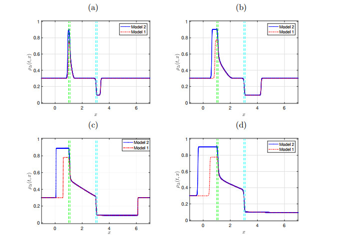
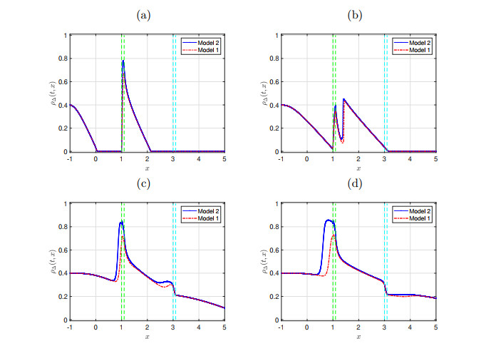
    Example 1. Numerical approximations of the problem (2.1). Dynamic of Model 1 vs. Model 2 at (a)T=0.5, (b)T=2, (c)T=5, (d)T=7

    .

    limit η0 in Model 2.

    In this example we take a look at the limit case η0 and investigate the convergence of the Model 2 to the solution of the local problem (1.1)-(1.3). In particular, we consider the initial condition ρ0(x)=0.3 for x[0,1], qon(t)=1.2, qoff(t)=0.8 at T=5 with fixed Δx=1/1000 and η{0.1,0.05,0.01,0.004}, and δ=0. To evaluate the convergence, we compute the L1 distance between the approximate solution obtained for the proposed upwind-type scheme by means Algorithm 3.1 with a given η and the result of a classical Godunov scheme for the corresponding local problem. In Table 1, we can observe that the L1 distance goes to zero when η0. The results are illustrated in Fig. 3.

    Table 1. 

    Example 2. L1 distance between the approximate solutions to the non-local problem and the local problem for different values of η at T=5 with Δx=1/1000

    .
    η 0.1 0.05 0.01 0.004
    L1 distance 2.8e-1 1.6e-1 3.6e-2 1.1e-2

     | Show Table
    DownLoad: CSV
    Figure 3. 

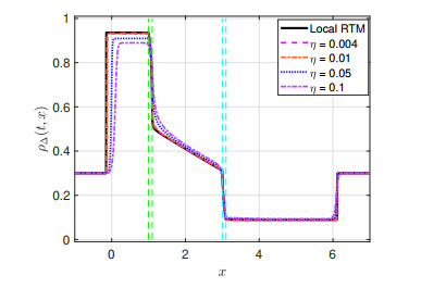
    Example 2. Numerical approximations of the problem (2.1) at T=5. Comparison of local and non-local versions of the model (2.1) with δ=0 and different values for η

    .

    Maximum principle.

    In this example we verify that the Algorithm 3.1 with the terms Son (3.2) and (3.3) satisfy the maximum principle, i.e., we verify numerically that Lemmas 1 and 5 respectively, are fulfilled. On the other hand, we also verify that the Algorithm 3.1 with a discretization of the term Son (1.4), which we called Model 0, does not satisfy a maximum principle. For this purpose we consider the initial condition given by

    ρ0(x)={0.1ifx1.11.0ifx>1.1,

    qon(t)=1, qoff(t)=0.2 at T=0.3, with Δx=1/100, η=0.05, and δ=0.01. We can see in Fig. 4 (a) that the Model 0 does not satisfy a maximum principle unlike Model 1 and Model 2. The Fig 4(b) is a zoom of (a) in which we can appreciate in a better form that Model 0 does not satisfy a maximum principle.

    Figure 4. 

    Example 3. Numerical approximation at time T=0.3. (a) Model 1, Model 2 satisfying a maximum principle and Model 0 not satisfying a maximum principle. (b) Zoom of a part of (a)

    .

    Free main road.

    In this example we consider a free main road, i.e, we consider a initial condition ρ0=0, boundary conditions ρ0(t)=0.4 for all t>0 and absorbing conditions at x=5. We also consider the rate of the on-ramp qon(t)=12(sin(πt)+1) and the rate of the off-ramp qoff(t)=0.2. We solve (2.1) numerically in the interval [1,5] in different times, namely T=1, T=2, T=5, T=7 and consider Δx=1/1000, η=0.1, δ=0.02. In Fig. 5 we can see the dynamic of the model 2.1 approximated by means of Model 1 and Model 2.

    Figure 5. 

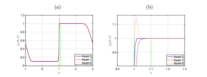
    Example 4. Dynamic of the model (2.1). Behavior of the numerical solution computed with Algorithm 3.1 by means of Model 1 and Model 2 at time (a)T=1, (b)T=2, (c)T=5, (d)T=7

    .

    In this paper we introduced a nonlocal balance law to model vehicular traffic flow including on- and off-ramps. We presented three different models called Model 0, Model 1 and Model 2 and we proved existence and uniqueness of solutions for Model 1 and Model 2. We approximated the problem through a upwind-type numerical scheme, providing a Maximum principle, L1 and BV estimates for approximate solutions. Numerical simulations illustrate the dynamics of the studied models and show that Model 0 does not satisfy a maximum principle. A limit model as the kernel support tends to zero is numerically investigated. In a future work, we would like to consider a nonlocal version of the second order model proposed in [21].

    FAC is member of GNFM (Gruppo Nazionale per la Fisica Matematica) of INdAM (Istituto Nazionale di Alta Matematica), Italy. LMV is supported by ANID-Chile through Fondecyt project 1181511 and by Centro de Modelamiento Matemático (CMM), ACE210010 and FB210005, BASAL funds for center of excellence from ANID-Chile. FAC, HDC and LMV are supported by the INRIA Associated Team "Efficient numerical schemes for non-local transport phenomena" (NOLOCO; 2018–2020) and by project MATH-Amsud 22-MATH-05 "NOTION: NOn-local conservaTION laws for engineering, biological and epidemiological applications: theoretical and numerical". HDC was partially supported by the National Agency for Research and Development, ANID-Chile through Scholarship Program, Doctorado Becas Chile 2021, 21210826.


    [1] On the numerical integration of scalar nonlocal conservation laws. ESAIM: Mathematical Modelling and Numerical Analysis (2015) 49: 19-37.
    [2]

    A. Bayen, A. Keimer, L. Pflug and T. Veeravalli, Modeling multi-lane traffic with moving obstacles by nonlocal balance laws, Preprint, (2020).

    [3] Well-posedness of a conservation law with non-local flux arising in traffic flow modeling. Numerische Mathematik (2016) 132: 217-241.
    [4] A non-local traffic flow model for 1-to-1 junctions. European Journal of Applied Mathematics (2020) 31: 1029-1049.
    [5] Global entropy weak solutions for general non-local traffic flow models with anisotropic kernel. ESAIM: Mathematical Modelling and Numerical Analysis (2018) 52: 163-180.
    [6] Non-local multi-class traffic flow models. Networks & Heterogeneous Media (2019) 14: 371-380.
    [7] A PDE-ODE model for a junction with ramp buffer. SIAM Journal on Applied Mathematics (2014) 74: 22-39.
    [8]

    J. Friedrich, S. Göttlich and E. Rossi, Nonlocal approaches for multilane traffic models, Commun. Math. Sci., 19 (2021), 2291–2317, arXiv preprint, arXiv: 2012.05794, (2020).

    [9] A godunov type scheme for a class of lwr traffic flow models with non-local flux. Networks & Heterogeneous Media (2018) 13: 531-547.
    [10] A multilane macroscopic traffic flow model for simple networks. SIAM Journal on Applied Mathematics (2019) 79: 1967-1989.
    [11] Well-posedness and finite volume approximations of the LWR traffic flow model with non-local velocity. Netw. Heterog. Media (2016) 11: 107-121.
    [12] Hierarchical ramp metering in freeways: An aggregated modeling and control approach. Transportation Research Part C: Emerging Technologies (2020) 110: 1-19.
    [13] Master: Macroscopic traffic simulation based on a gas-kinetic, non-local traffic model. Transportation Research Part B: Methodological (2001) 35: 183-211.
    [14] Models for dense multilane vehicular traffic. SIAM Journal on Mathematical Analysis (2019) 51: 3694-3713.
    [15] Optimal ramp metering strategy with extended lwr model, analysis and computational methods. IFAC Proceedings Volumes (2005) 38: 99-104.
    [16]

    G. Lipták, M. Pereira, B. Kulcsár, M. Kovács and G. Szederkényi, Traffic reaction model, arXiv preprint, arXiv: 2101.10190, (2021).

    [17] Modelling of freeway merging and diverging flow dynamics. Applied Mathematical Modelling (1996) 20: 459-469.
    [18] Stochastic modeling and simulation of traffic flow: Asymmetric single exclusion process with arrhenius look-ahead dynamics. SIAM Journal on Applied Mathematics (2006) 66: 921-944.
    [19] Study on traffic characteristics for a typical expressway on-ramp bottleneck considering various merging behaviors. Physica A: Statistical Mechanics and its Applications (2015) 440: 57-67.
    [20] Effects of the number of on-ramps on the ring traffic flow. Chinese Physics B (2010) 19: 050517.
    [21] A new macro model for traffic flow on a highway with ramps and numerical tests. Communications in Theoretical Physics (2009) 51: 71.
    [22] Congested traffic patterns of two-lane lattice hydrodynamic model with on-ramp. Nonlinear Dynamics (2017) 88: 1345-1359.
  • This article has been cited by:

    1. Harold Deivi Contreras, Paola Goatin, Luis-Miguel Villada, A two-lane bidirectional nonlocal traffic model, 2025, 543, 0022247X, 129027, 10.1016/j.jmaa.2024.129027
    2. Veerappa Gowda G. D., Sudarshan Kumar Kenettinkara, Nikhil Manoj, Convergence of a second-order scheme for non-local conservation laws, 2023, 57, 2822-7840, 3439, 10.1051/m2an/2023080
    3. Felisia A. Chiarello, Harold D. Contreras, 2024, Chapter 26, 978-3-031-55263-2, 303, 10.1007/978-3-031-55264-9_26
  • Reader Comments
  • © 2022 the Author(s), licensee AIMS Press. This is an open access article distributed under the terms of the Creative Commons Attribution License (http://creativecommons.org/licenses/by/4.0)
通讯作者: 陈斌, bchen63@163.com
  • 1. 

    沈阳化工大学材料科学与工程学院 沈阳 110142

  1. 本站搜索
  2. 百度学术搜索
  3. 万方数据库搜索
  4. CNKI搜索

Metrics

Article views(1623) PDF downloads(185) Cited by(3)

Figures and Tables

Figures(5)  /  Tables(1)

/

DownLoad:  Full-Size Img  PowerPoint
Return
Return

Catalog