We consider a homogenization problem for the diffusion equation $ -\operatorname{div}\left(a_{\varepsilon} \nabla u_{\varepsilon} \right) = f $ when the coefficient $ a_{\varepsilon} $ is a non-local perturbation of a periodic coefficient. The perturbation does not vanish but becomes rare at infinity in a sense made precise in the text. We prove the existence of a corrector, identify the homogenized limit and study the convergence rates of $ u_{\varepsilon} $ to its homogenized limit.
Citation: Rémi Goudey. A periodic homogenization problem with defects rare at infinity[J]. Networks and Heterogeneous Media, 2022, 17(4): 547-592. doi: 10.3934/nhm.2022014
We consider a homogenization problem for the diffusion equation $ -\operatorname{div}\left(a_{\varepsilon} \nabla u_{\varepsilon} \right) = f $ when the coefficient $ a_{\varepsilon} $ is a non-local perturbation of a periodic coefficient. The perturbation does not vanish but becomes rare at infinity in a sense made precise in the text. We prove the existence of a corrector, identify the homogenized limit and study the convergence rates of $ u_{\varepsilon} $ to its homogenized limit.

| [1] |
Homogenization and two-scale convergence. SIAM Journal on Mathematical Analysis (1992) 23: 1482-1518. 
|
| [2] |
Compactness methods in the theory of homogenization. Communications on Pure and Applied Mathematics (1987) 40: 803-847.
|
| [3] |
Compactness methods in the theory of homogenization II: Equations in non-divergence form. Communications on Pure and Applied Mathematics (1989) 42: 139-172.
|
| [4] |
$L^p$ bounds on singular integrals in homogenization. Communications on Pure and Applied Mathematics (1991) 44: 897-910.
|
| [5] |
A. Bensoussan, J.-L. Lions and G. Papanicolaou, Asymptotic Analysis for Periodic Structures, Studies in Mathematics and its Applications, 5. North-Holland Publishing Co., Amsterdam-New York, 1978. |
| [6] |
Precised approximations in elliptic homogenization beyond the periodic setting. Asymptotic Analysis (2020) 116: 93-137.
|
| [7] |
X. Blanc, C. Le Bris and P.-L. Lions, On correctors for linear elliptic homogenization in the presence of local defects: The case of advection-diffusion, Journal de Mathématiques Pures et Appliquées, 124 (2019), 106–122. |
| [8] |
On correctors for linear elliptic homogenization in the presence of local defects. Communications in Partial Differential Equations (2018) 43: 965-997.
|
| [9] |
Local profiles for elliptic problems at different scales: Defects in, and interfaces between periodic structures. Communications in Partial Differential Equations (2015) 40: 2173-2236.
|
| [10] |
A possible homogenization approach for the numerical simulation of periodic microstructures with defects. Milan Journal of Mathematics (2012) 80: 351-367.
|
| [11] |
Asymptotic behaviour of Green functions of divergence form operators with periodic coefficients. Applied Mathematics Research Express (2013) 2013: 79-101.
|
| [12] |
Les espaces du type de Beppo Levi. Annales de l'institut Fourier (1954) 5: 305-370.
|
| [13] |
L. C. Evans, Partial Differential Equations, Graduate Studies in Mathematics, 19. American Mathematical Society, Providence, RI, 1998. |
| [14] | (1983) Multiple Integrals in the Calculus of Variations and Nonlinear Elliptic Systems. Princeton University Press. |
| [15] |
M. Giaquinta and L. Martinazzi, An Introduction to the Regularity Theory for Elliptic Systems, Harmonic Maps and Minimal Graphs, Edizioni Della Normale, Pisa, 2012. |
| [16] |
R. Goudey, A periodic homogenization problem with defects rare at infinity, preprint, arXiv: 2109.05506. |
| [17] |
R. Goudey, PhD Thesis, in preparation. |
| [18] |
The Green function for uniformly elliptic equations. Manuscripta Mathematica (1982) 37: 303-342.
|
| [19] |
V. V. Jikov, S. M Kozlov and O. A. Oleinik, Homogenization of Differential Operators and Integral Functionals, Springer-Verlag, Berlin, 1994. |
| [20] |
P.-L. Lions, The concentration-compactness principle in the calculus of variations. The locally compact case, Parts 1 & 2, Annales de l'Institut Henri Poincaré C, Analyse non linéaire, 1 (1984), 109–145 and 223–283. |
| [21] |
L. Tartar, The General Theory of Homogenization: A Personalized Introduction, Springer, Berlin Heidelberger, 2009. |


Figures(3)
Rémi Goudey. A periodic homogenization problem with defects rare at infinity[J]. Networks and Heterogeneous Media, 2022, 17(4): 547-592. doi: 10.3934/nhm.2022014

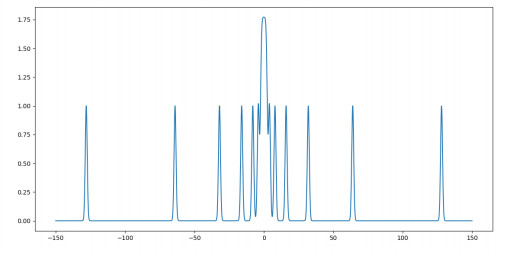
Prototype perturbation in dimension
Example of points in ambient dimension 2 that satisfy our assumptions along with their associated Voronoi diagram
Example for the choice of the open subset


 DownLoad: