We investigate existence of stationary solutions to an aggregation/diffusion system of PDEs, modelling a two species predator-prey interaction. In the model this interaction is described by non-local potentials that are mutually proportional by a negative constant $ -\alpha $, with $ \alpha>0 $. Each species is also subject to non-local self-attraction forces together with quadratic diffusion effects. The competition between the aforementioned mechanisms produce a rich asymptotic behavior, namely the formation of steady states that are composed of multiple bumps, i.e. sums of Barenblatt-type profiles. The existence of such stationary states, under some conditions on the positions of the bumps and the proportionality constant $ \alpha $, is showed for small diffusion, by using the functional version of the Implicit Function Theorem. We complement our results with some numerical simulations, that suggest a large variety in the possible strategies the two species use in order to interact each other.
Citation: Simone Fagioli, Yahya Jaafra. Multiple patterns formation for an aggregation/diffusion predator-prey system[J]. Networks and Heterogeneous Media, 2021, 16(3): 377-411. doi: 10.3934/nhm.2021010
We investigate existence of stationary solutions to an aggregation/diffusion system of PDEs, modelling a two species predator-prey interaction. In the model this interaction is described by non-local potentials that are mutually proportional by a negative constant $ -\alpha $, with $ \alpha>0 $. Each species is also subject to non-local self-attraction forces together with quadratic diffusion effects. The competition between the aforementioned mechanisms produce a rich asymptotic behavior, namely the formation of steady states that are composed of multiple bumps, i.e. sums of Barenblatt-type profiles. The existence of such stationary states, under some conditions on the positions of the bumps and the proportionality constant $ \alpha $, is showed for small diffusion, by using the functional version of the Implicit Function Theorem. We complement our results with some numerical simulations, that suggest a large variety in the possible strategies the two species use in order to interact each other.

| [1] |
L. Ambrosio, N. Gigli and G. Savaré, Gradient Flows in Metric Spaces and in the Space of Probability Measures, 2nd edition, Lectures in Mathematics ETH Zürich, Birkhäuser Verlag, Basel, 2008. |
| [2] |
Global minimizers for free energies of subcritical aggregation equations with degenerate diffusion. Applied Mathematics Letters (2011) 24: 1927-1932. 
|
| [3] |
N. Bellomo and S. -Y Ha, A quest toward a mathematical theory of the dynamics of swarms, Math. Models Methods Appl. Sci., 27 (2017), 745-770. |
| [4] |
N. Bellomo and J. Soler, On the mathematical theory of the dynamics of swarms viewed as complex systems, Math. Models Methods Appl. Sci., 22 (2012), 1140006. |
| [5] |
Large time behavior of nonlocal aggregation models with nonlinear diffusion. Netw. Heterog. Media (2008) 3: 749-785.
|
| [6] |
Sorting phenomena in a mathematical model for two mutually attracting/repelling species. SIAM J. Math. Anal. (2018) 50: 3210-3250.
|
| [7] |
M. Burger, M. Di Francesco and M. Franek, Stationary states of quadratic diffusion equations with long-range attraction, Commun. Math. Sci., 11 (2013), 709-738. |
| [8] |
M. Burger, R. Fetecau and Y. Huang, Stationary states and asymptotic behavior of aggregation models with nonlinear local repulsion, SIAM J. Appl. Dyn. Syst., 13 (2014), 397-424. |
| [9] |
Modeling the aggregative behavior of ants of the species polyergus rufescens}. Nonlinear Anal. Real World Appl. (2000) 1: 163-176.
|
| [10] |
Remarks on continuity equations with nonlinear diffusion and nonlocal drifts. J. Math. Anal. Appl. (2016) 444: 1690-1702.
|
| [11] |
Equilibria of homogeneous functionals in the fair-competition regime. Nonlinear Anal. (2017) 159: 85-128.
|
| [12] |
A finite-volume method for nonlinear nonlocal equations with a gradient flow structure. Commun. Comput. Phys. (2015) 17: 233-258.
|
| [13] |
Zoology of a nonlocal cross-diffusion model for two species. SIAM J. Appl. Math. (2018) 78: 1078-1104.
|
| [14] |
J. A. Carrillo and G. Toscani, Wasserstein metric and large-time asymptotics of nonlinear diffusion equations., New Trends in Mathematical Physics, World Sci. Publ., Hackensack, NJ, 2004, 234-244. |
| [15] |
Y. Chen and T. Kolokolnikov, A minimal model of predator-swarm interactions, J. R. Soc. Interface, 11 (2014). |
| [16] |
On minimizers of interaction functionals with competing attractive and repulsive potentials. Ann. Inst. H. Poincaré Anal. Non Linéaire (2015) 32: 1283-1305.
|
| [17] |
Ground states of a two phase model with cross and self attractive interactions. SIAM J. Math. Anal. (2016) 48: 3412-3443.
|
| [18] |
B. Düring, P. Markowich, J. -F. Pietschmann and M. -T. Wolfram, Boltzmann and Fokker-Planck equations modelling opinion formation in the presence of strong leaders, Proc. R. Soc. Lond. Ser. A Math. Phys. Eng. Sci. 465 (2009), 3687-3708. |
| [19] |
K. Deimling, Nonlinear Functional Analysis, Springer-Verlag, Berlin, 1985. |
| [20] |
Nonlinear degenerate cross-diffusion systems with nonlocal interaction. Nonlinear Anal. (2018) 169: 94-117.
|
| [21] |
A nonlocal swarm model for predators-prey interactions. Math. Models Methods Appl. Sci. (2016) 26: 319-355.
|
| [22] |
Measure solutions for non-local interaction PDEs with two species. Nonlinearity (2013) 26: 2777-2808.
|
| [23] |
M. Di Francesco, S. Fagioli, M. D. Rosini and G. Russo, Follow-the-Leader approximations of macroscopic models for vehicular and pedestrian flows, Active Particles, Vol. 1, Birkhäuser/Springer, Cham, 2017, 333-378. |
| [24] |
Multiple large-time behavior of nonlocal interaction equations with quadratic diffusion. Kinet. Relat. Models (2019) 12: 303-322.
|
| [25] |
Curves of steepest descent are entropy solutions for a class of degenerate convection-diffusion equations. Calc. Var. Partial Differential Equations (2014) 50: 199-230.
|
| [26] |
Y. Du, Order Structure and Topological Methods in Nonlinear Partial Differential Equations, Vol. 1, World Scientific Publishing Co. Pte. Ltd., Hackensack, NJ, 2006. |
| [27] |
J. Evers, R. Fetecau and T. Kolokolnikov, Equilibria for an aggregation model with two species, SIAM J. Appl. Dyn. Syst., 16 (2017), 2287-2338. |
| [28] |
Solutions to aggregation-diffusion equations with nonlinear mobility constructed via a deterministic particle approximation. Math. Models Methods Appl. Sci. (2018) 28: 1801-1829.
|
| [29] |
Stable stationary states of non-local interaction equations. Math. Models Methods Appl. Sci. (2010) 20: 2267-2291.
|
| [30] |
Stability of stationary states of non-local equations with singular interaction potentials. Math. Comput. Modelling (2011) 53: 1436-1450.
|
| [31] |
Strong stability-preserving high-order time discretization methods. SIAM Rev. (2001) 43: 89-112.
|
| [32] |
S. Guo, Bifurcation and spatio-temporal patterns in a diffusive predator-prey system, Nonlinear Anal. Real World Appl., 42 (2018), 448-477. |
| [33] |
The variational formulation of the Fokker-Planck equation. SIAM J. Math. Anal. (1998) 29: 1-17.
|
| [34] |
Stationary states of an aggregation equation with degenerate diffusion and bounded attractive potential. SIAM J. Math. Anal. (2017) 49: 272-296.
|
| [35] | (2002) Living in Groups. Oxford University Press. |
| [36] |
Contribution to the theory of periodic reaction. J. Phys. Chem. (1910) 14: 271-274.
|
| [37] |
A family of nonlinear fourth order equations of gradient flow type. Comm. Partial Differential Equations (2009) 34: 1352-1397.
|
| [38] |
M. Mimura and M. Yamaguti, Pattern formation in interacting and diffusing systems in population biology, Adv. Biophys. 15, 19-65, 1982. |
| [39] |
A non-local model for a swarm. J. Math. Biol. (1999) 38: 534-570.
|
| [40] |
D. Morale, V. Capasso and K. Oelschläger, An interacting particle system modelling aggregation behavior: From individuals to populations, J. Math. Biol., 50 (2005), 49-66. |
| [41] |
J. D. Murray, Mathematical Biology. I, 3rd edition, Interdisciplinary Applied Mathematics, Vol. 17, Springer-Verlag, New York, 2002. |
| [42] |
A. Okubo and S. A. Levin, Diffusion and Ecological Problems: Modern Perspectives, 2nd edition, Interdisciplinary Applied Mathematics, Vol. 14, Springer-Verlag, New York, 2001. |
| [43] |
Complexity, patterns and evolutionary trade-offs in animal aggregation. Science (1999) 254: 99-101.
|
| [44] | Tightness, integral equicontinuity and compactness for evolution problems in Banach spaces. Ann. Sc. Norm. Super. Pisa Cl. Sci. (5) (2003) 2: 395-431. |
| [45] |
F. Santambrogio, Optimal Transport for Applied Mathematicians, Progress in Nonlinear Differential Equations and Their Applications, Vol. 87, Birkhäuser/Springer, Cham, 2015. |
| [46] |
H. Tomkins and T. Kolokolnikov, Swarm shape and its dynamics in a predator-swarm model, preprint, 2014. |
| [47] |
Swarming patterns in a two-dimensional kinematic model for biological groups. SIAM J. Appl. Math. (2004) 65: 152-174.
|
| [48] |
A nonlocal continuum model for biological aggregation. Bull. Math. Biol. (2006) 68: 1601-1623.
|
| [49] |
M. Torregrossa and G. Toscani, On a Fokker-Planck equation for wealth distribution, Kinet. Relat. Models, 11 (2018), 337-355. |
| [50] |
M. Torregrossa and G. Toscani, Wealth distribution in presence of debts. A Fokker-Planck description, Commun. Math. Sci., 16 (2018), 537-560. |
| [51] |
G. Toscani, Kinetic models of opinion formation, Commun. Math. Sci., 4 (2006), 481-496. |
| [52] | (2007) The Porous Medium Equation. Mathematical Theory. Oxford University Press, Oxford: Oxford Mathematical Monographs, The Clarendon Press. |
| [53] |
C. Villani, Topics in Optimal Transportation, Graduate Studies in Mathematics, Vol. 58, American Mathematical Society, Providence, RI, 2003. |
| [54] | Variazioni e fluttuazioni del numero d'individui in specie animali conviventi. Mem. Accad. Lincei Roma (1926) 2: 31-113. |


Figures(9)
Simone Fagioli, Yahya Jaafra. Multiple patterns formation for an aggregation/diffusion predator-prey system[J]. Networks and Heterogeneous Media, 2021, 16(3): 377-411. doi: 10.3934/nhm.2021010

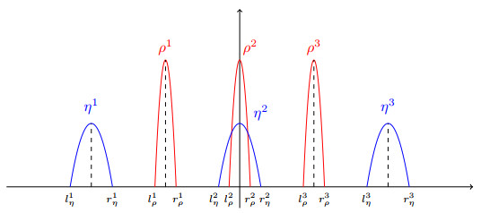
A possible example of a stationary solution to (3) with
Example of mixed stationary state. Note that by symmetry
An example of a separated stationary state
In this figure, a mixed steady state is plotted by using initial data given by (70),
A separated steady state is presented in this figure. Initial data are given by (71). The parameters are
This figure shows how from the initial densities
A steady state of four bumps is showed in this figure starting from initial data as in (72) with
Starting from initial data as in (73) with
This last figure shows a possible existence of traveling waves by choosing initial data as in (74),


 DownLoad: