Entropy-preserving coupling conditions for one-dimensional Euler systems at junctions

  • Received: 01 April 2017 Revised: 01 September 2017
  • Primary: 35L60, 35L65, 35Q31, 35R02, 76N10

  • This paper is concerned with a set of novel coupling conditions for the 3× 3 one-dimensional Euler system with source terms at a junction of pipes with possibly different cross-sectional areas. Beside conservation of mass, we require the equality of the total enthalpy at the junction and that the specific entropy for pipes with outgoing flow equals the convex combination of all entropies that belong to pipes with incoming flow. Previously used coupling conditions include equality of pressure or dynamic pressure. They are restricted to the special case of a junction having only one pipe with outgoing flow direction. Recently, Reigstad [SIAM J. Appl. Math., 75:679-702,2015] showed that such pressure-based coupling conditions can produce non-physical solutions for isothermal flows through the production of mechanical energy. Our new coupling conditions ensure energy as well as entropy conservation and also apply to junctions connecting an arbitrary number of pipes with flexible flow directions. We prove the existence and uniqueness of solutions to the generalised Riemann problem at a junction in the neighbourhood of constant stationary states which belong to the subsonic region. This provides the basis for the well-posedness of the homogeneous and inhomogeneous Cauchy problems for initial data with sufficiently small total variation.

    Citation: Jens Lang, Pascal Mindt. 2018: Entropy-preserving coupling conditions for one-dimensional Euler systems at junctions, Networks and Heterogeneous Media, 13(1): 177-190. doi: 10.3934/nhm.2018008

    Related Papers:

    [1] Jens Lang, Pascal Mindt . Entropy-preserving coupling conditions for one-dimensional Euler systems at junctions. Networks and Heterogeneous Media, 2018, 13(1): 177-190. doi: 10.3934/nhm.2018008
    [2] Gunhild A. Reigstad . Numerical network models and entropy principles for isothermal junction flow. Networks and Heterogeneous Media, 2014, 9(1): 65-95. doi: 10.3934/nhm.2014.9.65
    [3] Gabriella Bretti, Roberto Natalini, Benedetto Piccoli . Numerical approximations of a traffic flow model on networks. Networks and Heterogeneous Media, 2006, 1(1): 57-84. doi: 10.3934/nhm.2006.1.57
    [4] Martin Gugat, Alexander Keimer, Günter Leugering, Zhiqiang Wang . Analysis of a system of nonlocal conservation laws for multi-commodity flow on networks. Networks and Heterogeneous Media, 2015, 10(4): 749-785. doi: 10.3934/nhm.2015.10.749
    [5] Steinar Evje, Kenneth H. Karlsen . Hyperbolic-elliptic models for well-reservoir flow. Networks and Heterogeneous Media, 2006, 1(4): 639-673. doi: 10.3934/nhm.2006.1.639
    [6] Michael Herty, S. Moutari, M. Rascle . Optimization criteria for modelling intersections of vehicular traffic flow. Networks and Heterogeneous Media, 2006, 1(2): 275-294. doi: 10.3934/nhm.2006.1.275
    [7] Michael Herty, Niklas Kolbe, Siegfried Müller . Central schemes for networked scalar conservation laws. Networks and Heterogeneous Media, 2023, 18(1): 310-340. doi: 10.3934/nhm.2023012
    [8] Rinaldo M. Colombo, Francesca Marcellini . Coupling conditions for the $3\times 3$ Euler system. Networks and Heterogeneous Media, 2010, 5(4): 675-690. doi: 10.3934/nhm.2010.5.675
    [9] Dilip Sarkar, Shridhar Kumar, Pratibhamoy Das, Higinio Ramos . Higher-order convergence analysis for interior and boundary layers in a semi-linear reaction-diffusion system networked by a $ k $-star graph with non-smooth source terms. Networks and Heterogeneous Media, 2024, 19(3): 1085-1115. doi: 10.3934/nhm.2024048
    [10] Jan Friedrich, Simone Göttlich, Annika Uphoff . Conservation laws with discontinuous flux function on networks: a splitting algorithm. Networks and Heterogeneous Media, 2023, 18(1): 1-28. doi: 10.3934/nhm.2023001
  • This paper is concerned with a set of novel coupling conditions for the 3× 3 one-dimensional Euler system with source terms at a junction of pipes with possibly different cross-sectional areas. Beside conservation of mass, we require the equality of the total enthalpy at the junction and that the specific entropy for pipes with outgoing flow equals the convex combination of all entropies that belong to pipes with incoming flow. Previously used coupling conditions include equality of pressure or dynamic pressure. They are restricted to the special case of a junction having only one pipe with outgoing flow direction. Recently, Reigstad [SIAM J. Appl. Math., 75:679-702,2015] showed that such pressure-based coupling conditions can produce non-physical solutions for isothermal flows through the production of mechanical energy. Our new coupling conditions ensure energy as well as entropy conservation and also apply to junctions connecting an arbitrary number of pipes with flexible flow directions. We prove the existence and uniqueness of solutions to the generalised Riemann problem at a junction in the neighbourhood of constant stationary states which belong to the subsonic region. This provides the basis for the well-posedness of the homogeneous and inhomogeneous Cauchy problems for initial data with sufficiently small total variation.


    We consider the one-dimensional polytropic Euler equations with source terms at a network with one single junction connecting $N$ pipe sections of infinite length

    $ \partial_t U^{(i)} + \partial_x F(U^{(i)}) = G(x, t, U^{(i)}), (x, t)\in\mathbb{R}^+\times\mathbb{R}^+, $ (1)
    $ U^{(i)}(x, 0) = U^{(i)}_0(x), x\in \mathbb{R}^+, $ (2)

    for $i = 1, \ldots, N$, with the thermodynamic variables and the flux functions

    $ \label{euler_flux} U^{(i)} = (ρiρiuiEi)
    \;\;\mbox{and}\;\; F(U^{(i)}) = (ρiuiρiu2i+piui(Ei+pi))
    . $
    (3)

    Each pipe is described by a vector, $\nu_i\in\mathbb{R}^3\setminus\{0\}$, originating from the common junction and parameterized by $x\in\mathbb{R}^+$, the real halfline $[0, \infty)$. The surface section of the pipe equals $\|\nu_i\|\!\ne\!0$. We assume $\nu_i\ne \nu_j$ for $i\ne j$. Further, $\rho_i$ is the density, $u_i$ is the velocity, $p_i$ is the pressure, and $E_i$ is the total energy. The equation of state for an ideal polytropic gas in the common form reads

    $ E_i = \frac{p_i}{\gamma-1} + \frac12 \rho_iu_i^2 $ (4)

    with a suitable adiabatic exponent $\gamma>1$. For later use, we introduce the mass flux, $q_i = \rho_iu_i$, the speed of sound, $c_i = \sqrt{\gamma p_i/\rho_i}$, as well as the specific entropy $s_i$ and the total enthalpy $h_i$ defined by

    $ s_i = c_v\, \ln\left( \frac{p_i}{\rho_i^\gamma}\right) \;\;\mbox{and}\;\; h_i = \frac{E_i+p_i}{\rho_i} $ (5)

    with the specific (constant) heat capacity $c_v>0$. More details about the underlying thermodynamic principles can be found, e.g., in [14,Sect.14.4]. The right-hand side vector $G(x, t, U^{(i)})$ describes source terms, e.g., gravity and friction. We will first discuss the homogeneous case $G = 0$, yielding a system of conservation laws in (1), and extend our results to the inhomogeneous case later on through operator splitting techniques, following known concepts.

    The characteristic eigenvalues of the Euler equations are

    $ \lambda_1(U) = u - c, \;\; \lambda_2(U) = u, \;\; \lambda_3(U) = u + c. $ (6)

    As usual in the literature, we also restrict our analysis to the subsonic region defined by $|u| <c$, and introduce the two sets of subsonic data

    $ D^+ : = \{ U = (\rho, \rho u, E)\in \overset{{}^\circ }{\mathop{\mathbb{R}}}\,^+\times\mathbb{R}\times\overset{{}^\circ }{\mathop{\mathbb{R}}}\,^+: \, \lambda_1(U) < 0 < \lambda_2(U) < \lambda_3(U)\}, $ (7)
    $ D^- : = \{ U = (\rho, \rho u, E)\in\overset{{}^\circ }{\mathop{\mathbb{R}}}\,^+\times\mathbb{R}\times\overset{{}^\circ }{\mathop{\mathbb{R}}}\,^+: \, \lambda_1(U) < \lambda_2(U) < 0 < \lambda_3(U)\}, $ (8)

    with $\overset{{}^\circ }{\mathop{\mathbb{R}}}\,^+ = (0, \infty)$. Due to $\lambda_2(U) = u$ and the orientation of the pipes, we can relate pipes with a flow direction towards the junction with $D^-$ (incoming flow), while $D^+$ corresponds to pipes with flow direction away from the junction (outgoing flow). The corresponding index sets are defined by $\mathbb{I}_{i}: = \{i:U^{(i)}\in D^-\}$ and $\mathbb{I}_{o}: = \{i:U^{(i)}\in D^+\}$. We will only consider cases with $\mathbb{I}_i\cup\mathbb{I}_o = \{1, \ldots, N\}$.

    The main challenge in network modelling is to prescribe a set of coupling conditions at the junction-pipe interfaces of the form

    $ \Phi \left( U^{(1)}(0^+, t), \ldots, U^{(N)}(0^+, t) \right) = \Pi(t), $ (9)

    where $\Phi$ is a possibly nonlinear function of the traces $U^{(i)}(0^+, t) = \lim_{x\rightarrow 0^+}U^{(i)}(x, t)$ of the unknown variables and $\Pi$ is a coupling constant, which depends only on time. The conditions are closely linked to the Euler equations (1) and provide a relation between the flows in all pipes. Various functions $\Phi$ have been proposed in the literature. We find

    $ (M)Ni=1νiqi(0+,t)=0,t>0(conservation of mass), (E)Ni=1νi(ui(Ei+pi))(0+,t)=0,t>0(conservation of energy), (P)pi(0+,t)=p(t),t>0(equality of pressure), (PD)(ρiu2i+pi)(0+,t)=P(t),t>0(equality of dynamic pressure), (H)hi(0+,t)=h(t),t>0(equality of enthalpy), (S)Ni=1νi(qisi)(0+,t)0,t>0(entropy increase), 
    $

    where $p^*(t)$, $P^*(t)$ and $h^*(t)$ are unique, scalar, momentum-and enthalpy-related coupling constants, respectively. Note that the dynamic pressure in $(P_D)$ equals the momentum flux in (3).

    Colombo and Mauri [10] used coupling conditions that include mass and energy conservation at the junction, the equality of dynamic pressure as well as the entropy increase, i.e., the trace of the solution satisfies $(M)$, $(E)$, $(P_D)$, and $(S)$. They proved the well-posedness of the Cauchy problem given by the equations (1), (2), and (9) above, under the standard condition that the total variation of the initial data is sufficiently small. The proof was given for the special case of $\mathbb{I}_o = \{1\}$ and $\mathbb{I}_i = \{2, \ldots, N\}$, i.e., one pipe with outgoing flow and incoming flow in the remaining $N\!-\!1$ pipes. Herty [13] replaced the coupling condition $(P_D)$ by the equality of pressure, $(P)$, widely used in the engineering community to simulate gas networks. Following the approach presented in [10], he also showed well-posedness of the Cauchy problem for the special network studied there. However, the comparison to two-dimensional numerical results did not give a conclusion on whether dynamic pressure or pressure is the most appropriate momentum-related coupling constant. The one-dimensional coupling of two systems of Euler equations at a fixed interface were studied by Chalons, Raviart and Seguin in [4]. They discussed possible solutions to coupled Riemann problems for three different types of coupling conditions. Colombo and Marcellini [9] investigated the coupling of two pipes with different cross sectional areas and extended their results to a more complex pipe with spatially varying cross sectional area. An important and necessary assumption is the bounded total variation of the pipe's area profile. Physically motivated coupling conditions for tunnel fires in networks were formulated by Gasser and Kraft [12]. They considered the small Mach number regime and assumed a good mixing of the flow in the junction, which motivates conservation of mass and internal energy, the equality of pressure and an equal inflow condition for all densities of outgoing tunnels.

    Pressure equality, $(P)$, as coupling condition for isothermal flow in pipeline networks have been intensively studied by Banda, Herty and Klar [2,1]. Recently, Reigstad [17] (see also [15,16,18]) showed for this type of flow that both coupling conditions $(P)$ and $(P_D)$ deliver non-physical solutions characterized by the production of mechanical energy at a junction in a constructed test case with $N\! = \!3$. The main result of the paper comprises the fact that only the Bernoulli invariant taken as momentum-related coupling constant is proved to yield entropic solutions for all subsonic flow conditions in the general case of a junction connecting $N$ pipes of arbitrary cross-sectional area. The Bernoulli invariant equals the specific stagnation enthalpy and thus can be seen as the enthalpy-related coupling constants $h^*(t)$ in condition $(H)$ above. Together with the conservation of mass and the relation $q_ih_i\! = \!u_i(E_i+p_i)$, the equality of enthalpy at the junction immediately yields the conservation of energy. Thus, $(M)$ and $(H)$ imply $(E)$ for the Euler system. In this sense, the equality of enthalpy at the junction confirms the energy conservation there and represents a first step towards answering the main question of how to close the set of coupling conditions.

    In contrast to the isothermal flow, the situation for the compressible Euler equations with subsonic flow conditions is still unsettled and the analysis suffers from the open question: What are further physically sound coupling conditions for which well-posedness of Cauchy problems can be shown for the general case of a junction connecting $N$ pipes of arbitrary cross-sectional area and flexible flow directions? A common approach to tackle this question is to consider a generalised Riemann problem at the junction. Suppose we ensure mass conservation and the continuity of the enthalpy, i.e., $(M)$ and $(H)$ hold. Then, a closer inspection of the local solution structure of the Riemann problem and the corresponding degrees of freedom (as done in Sect. 2) shows that only one further coupling condition can be imposed for each of the outgoing pipes. This observation also explains the choice of the special network in [10,13]. There, $(P)$ or $(P_D)$ were chosen instead of $(H)$, and the conservation of energy was added, which allows to only consider one outgoing pipe.

    In this paper, we consider the equality of the entropy at the junction-pipe interface for pipes with outgoing flow:

    $ (S_o) \;\;\;\; s_i(0^+, t) = s^*(t), \;t > 0, \;i\in\mathbb{I}_o \;\; \mbox{(equality of outgoing entropy)}, $ (10)

    where the coupling constant $s^*(t)$ is identified as the convex combination of all entropies that belong to the pipes with incoming flow. That is, we set

    $ (S_i) \;\;\;\; {\displaystyle s^*(t) = \frac{1}{\sum\limits_{i\in\mathbb{I}_i}\, \|\nu_i\|q_i(0^+, t)} \, \sum\limits_{i\in\mathbb{I}_i}\, \|\nu_i\|(q_is_i)(0^+, t)} \;\;\; \mbox{(entropy mix)}. $ (11)

    Our choice is motivated by the assumption that gas flows entering a junction mix perfectly, which was also used by Schmidt, Steinbach, and Willert [19] to derive a mixing temperature at junctions and by Gasser and Kraft [12] to formulate an equal inflow boundary condition for all densities of outgoing pipes. A direct consequence of (11) and the conservation of mass is the conservation of entropy per unit volume in smooth flows. In this case, the momentum equation in (1) can be equivalently reformulated to $\partial_t(\rho s)+ \partial_x(qs)\! = \!0$ (see, e.g., [14,Sect.14.5]). Thanks to (11), we have the identity $\sum_{i\in\mathbb{I}_i}\, \|\nu_i\|(q_is_i)(0^+, t) = s^*(t)\sum_{i\in\mathbb{I}_i}\, \|\nu_i\|q_i(0^+, t)$, and therefore

    $ (S') \;\;\;\; \sum\limits_{i = 1}^{N}\, \|\nu_i\|\, (q_is_i)(0^+, t) = 0, \;t > 0 \;\;\; \mbox{(entropy conservation}). $ (12)

    The paper is organised as follows. In Sect. 2, we formulate the generalised Riemann problem at a junction with the coupling conditions $(M)$, $(H)$, $(S_o)$, $(S_i)$ and show its well-posedness. The corresponding Cauchy problem and its solution are studied in Sect. 3. A summary is given in Sect. 4.

    In this section, we show the well-posedness of the coupling conditions $(M)$, $(H)$, $(S_o)$, and $(S_i)$ for the homogeneous problem given by (1) with $G\! = \!0$. To this end, we consider a generalised Riemann problem at a junction and show that there exist a unique self-similar solution in terms of the classical Lax solution to standard Riemann problems. The theoretical framework was introduced by Colombo and Garavello [5] for the $p$-system and generalised in [10] to Euler systems.

    Let denote by $\Omega_i = \{U^{(i)}\in\mathbb{R}^3:\rho_i>0, \, p_i>0\}$ nonempty sets and define the overall state space $\Omega = \Omega_1\times\Omega_2\times\cdots\times\Omega_N$. Furthermore, let $Y = (Y^{(1)}, \ldots, Y^{(N)})$.

    We first recall two basic definitions for generalised Riemann problems at junctions.

    Definition 2.1. The Riemann problem at a junction with $N$ pipes is defined through the set of equations

    $ tY(i)+xF(Y(i))=0,(x,t)R+×R+,Φ(Y(1)(0+,t),,Y(N)(0+,t))=ˉΠ,Y(i)(x,0)=ˉY(i)0,xR+,
    $
    (13)

    for $i = 1, \ldots, N$, where $\bar{Y}^{(1)}_0, \ldots, \bar{Y}^{(N)}_0$ are constant thermodynamic states in $\Omega$ and $\bar{\Pi}\in\mathbb{R}^d$ is also constant.

    Definition 2.2. A $\Phi$-solution to the Riemann problem (13) is a self-similar function $Y(x, t):\mathbb{R}^+\times\mathbb{R}^+\rightarrow\Omega$ for which the following hold:

    1. There exists a constant state $Y_\ast(\bar{Y}_0) = \lim_{x\rightarrow 0^+}Y(x, t)$ such that all components $Y^{(i)}(x, t)$ coincide with the restriction to $x>0$ of the Lax solution to the standard Riemann problem for $x\in\mathbb{R}$,

    $ \label{prob_crm} \begin{array}{rll}
    \partial_t Y^{(i)} + \partial_x F(Y^{(i)}) & = & 0, \\
    Y^{(i)}(x, 0) & = & \left\{
     \begin{array}{ll}
     \bar{Y}^{(i)}_0 & \mbox{if }x > 0, \\
     Y^{(i)}_\ast & \mbox{if }x < 0.
     \end{array}
    \right. \end{array} $
    (14)

    2. The state $Y_\ast$ satisfies $\Phi(Y_\ast) = \bar{\Pi}$ for all $t>0$.

    The solution of the standard Riemann problem (14) with initial data $(U_L, U_R)$ for $x<0$ and $x>0$, respectively, can be described by a set of elementary waves such as rarefaction, contact and shock waves. The three waves separate four constant states $(U_L, U_{L\ast}, U_{R\ast}, U_R)$. The structure of the Euler equations reveals that the middle $2$-wave is always a contact discontinuity while the left and right waves can be either shock or rarefaction waves, see Fig. 1. Further, both the velocity and the pressure are constant across the contact discontinuity, i.e., it holds

    Figure 1. 

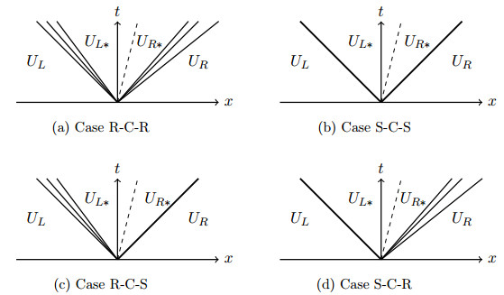
    Possible wave patterns in the solution of Riemann problems for the Euler equations: shock (S), contact (C) and rarefaction (R).

    .
    $ p_\ast = p_{L\ast} = p_{R\ast} \;\;\;\mbox{ and }\;\;\; u_\ast = u_{L\ast} = u_{R\ast}. $ (15)

    The four sought (constant) variables $(p_\ast, u_\ast, \rho_{L\ast}, \rho_{R\ast})$ are implicitly defined by means of parametrisations of the Rankine-Hugoniot jump condition and the Riemann invariants, see [20,Sect.4] or [14,Sect.14.11] for more details. We have

    $ u_\ast = u_L-\psi(p_\ast, U_L) = u_R+\psi(p_\ast, U_R), $ (16)
    $ \rho_{L\ast} = \phi(p_\ast, U_L), \;\;\; \rho_{R\ast} = \phi(p_\ast, U_R), $ (17)

    where for $k = L, R$,

    $ \psi(p_\ast, U_k) = {2ckγ1((ppk)γ12γ1)if ppk (rarefaction)(ppk)(1μ2ρk(p+μ2pk))12if p>pk (shock)
    $
    (18)
    $ \phi(p_\ast, U_k) = {ρk(ppk)1γif ppk (rarefaction)ρkp+μ2pkμ2p+pkif p>pk (shock)
    $
    (19)

    with $\mu^2 = (\gamma-1)/(\gamma+1)$ and $c_k^2 = \gamma p_k/\rho_k$. Observe that the second equality in (16) is used to determine the parameter $p_\ast$. The functions $\psi(p_\ast, U_k)$ and $\phi(p_\ast, U_k)$ are twice continuously differentiable at $p_\ast = p_k$. The total energy for the inner region can be computed from $E_{k\ast} = p_\ast/(\gamma-1)+\rho_{k\ast}u_{\ast}^2/2$ for $k = L, R$.

    For later use, let $\mathcal{L}_1(\sigma, U_L)$ denote the $1$-Lax curve, which parameterizes the $1$-wave curve through the state $U_L$ and describes all physical states on the right that can be reached from $U_L$ by either a shock wave for $\sigma>p_L$ or a rarefaction wave for $\sigma\le p_L$. Using (16) and (17), $\mathcal{L}_1$ is defined through

    $ \mathcal{L}_1(\sigma, U_L) : = (ϕ(σ,UL)ϕ(σ,UL)(uLψ(σ,UL))σγ1+12ϕ(σ,UL)(uLψ(σ,UL))2)
    $
    (20)

    Analogously, let $\mathcal{L}_3(\sigma, U_R)$ denote the $3$-Lax curve through the state $U_R$, defined through

    $ \mathcal{L}_3(\sigma, U_R) : = (ϕ(σ,UR)ϕ(σ,UR)(uR+ψ(σ,UR))σγ1+12ϕ(σ,UR)(uR+ψ(σ,UR))2)
    $
    (21)

    We further recall the fact that for the $2$-contact discontinuity, any state

    $ \mathcal{L}_2(\tau, \bar{U}) : = \bar{U} + \tau \left( 1, \, \bar{u}, \, \frac{1}{2}\bar{u}^2\right)^T $ (22)

    can be connected to $\bar{U}$ for sufficiently small $\tau\in\mathbb{R}$. This defines the $2$-Lax curve.

    We can now express the coupling conditions for the $\Phi$-solution to the Riemann problem (13) in terms of the Lax curves. Remember that in our network modelling, the $x$-coordinates are chosen in such a way that pipes are only outgoing from a junction. Consequently, switching from the standard to the generalised Riemann problem, the sign for the velocity in incoming pipes has to be changed. This changes the parametrisation of the $\mathcal{L}_1$-curve in (20). A closer inspection of (16) shows that $\mathcal{L}_1$ has to be replaced by $\mathcal{L}_3$.

    Due to the special parametrisation of the pipes and the restriction to subsonic flow, the contact discontinuity always travels with positive wave speed and, hence, the state $Y_\ast$ from (14) lies in the region $L_\ast$, see Fig. 2. We first parameterize all states $Y^{(i)}_{L\ast}$ using $\mathcal{L}_3$ for incoming pipes and $\mathcal{L}_2\circ\mathcal{L}_3$ for outgoing pipes, and then apply the function $\Phi$ to them. This yields the set of equations

    Figure 2. 

    Connection of the regions $L$, $L\ast$, $R\ast$, and $R$ with the Lax curve $\mathcal{L}_3$ for incoming pipes (a) and the Lax curves $\mathcal{L}_2\!\circ\!\mathcal{L}_3$ for outgoing pipes (b).

    .
    $ \Phi\left(\left( Y^{(i)}_{L\ast}\right)_{i\in\mathbb{I}_i}, \, \left( Y^{(j)}_{L\ast}\right)_{j\in\mathbb{I}_o}\right) = \bar{\Pi}\in\mathbb{R}^d $ (23)

    with

    $ Y^{(i)}_{L\ast} = \mathcal{L}_3(\sigma_i, \bar{Y}^{(i)}_0), \;i\in\mathbb{I}_i, \;\;\;\mbox{and}\;\;\; Y^{(j)}_{L\ast} = \mathcal{L}_2(\tau_j, \mathcal{L}_3(\sigma_j, \bar{Y}^{(j)}_0)), \;j\in\mathbb{I}_o. $ (24)

    Let $N_o = \dim(\mathbb{I}_o)$. Then, the degrees of freedom defined by the Lax curves are $\sigma = (\sigma_1, \ldots, \sigma_N)$ and $\tau = (\tau_1, \ldots, \tau_{N_o})$. Obviously, to ensure well-posedness of the generalised Riemann problem at a junction, one coupling condition has to be provided for incoming pipes, whereas two conditions are necessary for each of the outgoing pipes. The overall dimension of the parameter space is $d = N+N_o$.

    Given constant states $\bar{Y}^{(i)}_0\in D^+, i\! = \!1, \ldots, N_o$, and $\bar{Y}^{(j)}_0\in D^-, j\! = \!N_o+1, \ldots, N$, mass flux, enthalpy and entropy for the $L_\ast$-region can be extracted from formula (24):

    $ \label{eq_qhs} fi(σi,τi)=fi(L2(τi,L3(σi,ˉY(i)0))),i=1,,No,fj(σj)=fj(L3(σj,ˉY(j)0)),j=No+1,,N,
    $
    (25)

    with $f = q, h, s$. In what follows, we will consider the following coupling conditions taken from $(M)$, $(H)$, $(S_o)$, and $(S_i)$:

    $ 0 = \Phi(\sigma, \tau) = (i=1,,Noνiqi(σi,τi)+j=No+1,,Nνjqj(σj)hNo+1(σNo+1)h1(σ1,τ1)hNo+1(σNo+1)hNo(σNo,τNo)hNo+1(σNo+1)hNo+2(σNo+2)hNo+1(σNo+1)hN(σN)s1(σ1,τ1)s(σNo+1,,σN)sNo(σNo,τNo)s(σNo+1,,σN))
    $
    (26)

    with $s^\ast$ defined through

    $ s^\ast = \frac{1}{\sum_{j = N_o+1, \ldots, N}\, \|\nu_j\|q_j(\sigma_j)} \, \sum\limits_{j = N_o+1, \ldots, N}\, \|\nu_j\|(q_js_j)(\sigma_j). $ (27)

    The regularity of the Lax curves ensures the property $\Phi\in C^1(\mathbb{R}^N\times\mathbb{R}^{N_o}, \mathbb{R}^d)$. It remains to show that (26) has a unique solution. Then, Newton's method is applied to determine the solution vector $(\sigma^\ast, \tau^\ast)$, which finally gives the desired state $Y_\ast$ from

    $ Y^{(i)}_\ast = \mathcal{L}_3(\sigma_i^\ast, \bar{Y}^{(i)}_0), \;i\in\mathbb{I}_i, \;\;\mbox{and}\;\; Y^{(j)}_\ast = \mathcal{L}_2(\tau_j^\ast, \mathcal{L}_3(\sigma_j^\ast, \bar{Y}^{(j)}_0)), \;j\in\mathbb{I}_o. $ (28)

    We note that due to the special choice in (26) energy and entropy are conserved at the junction, i.e., $(E)$ and $(S')$ are fulfilled with $Y_\ast$.

    In the case $N = 2$ and parallel pipes with the same surface section, the solution of the generalised Riemann problem coincides with the solution of the standard Riemann problem for the polytropic Euler equations. We have

    Lemma 2.3. Let $N\! = \!2$, $\nu_1\! = \!-\nu_2\ne 0$, and assume constant initial data $(\bar{\rho}_1, \bar{q}_1, \bar{E}_1) \in D^+$ and $(\bar{\rho}_2, \bar{q}_2, \bar{E}_2)\in D^-$. Let $U(x, t)$ be the solution to the standard Riemann problem for (1) with initial data

    $ U(x, 0) = (\rho, q, E)(x, 0) = {(ˉρ1,ˉq1,ˉE1)forx>0,(ˉρ2,ˉq2,ˉE2)forx<0.
    $
    (29)

    Then the functions

    $ Y(1)(x,t)=(ρ1,q1,E1)(x,t)=(ρ,q,E)(x,t)ifx>0,Y(2)(x,t)=(ρ2,q2,E2)(x,t)=(ρ,q,E)(x,t)ifx<0
    $
    (30)

    are $\Phi$-solutions in the sense of Def. 2.2 that satisfy the coupling conditions (26). And vice versa, if $Y^{(i)}(x, t), i\! = \!1, 2, $ are such solutions, then $U(x, t)$ is the solution of the standard Riemann problem with initial data (29).

    Proof. Observe that the assertion holds true if the following equivalence is satisfied: $\Phi(Y^{(1)}_{L\ast}, Y^{(2)}_{L\ast})\! = \!0$ if and only if $(\rho^{(1)}_{L\ast}, q^{(1)}_{L\ast}, E^{(1)}_{L\ast})\! = \!(\rho^{(2)}_{L\ast}, -q^{(2)}_{L\ast}, E^{(2)}_{L\ast})$. The coupling conditions simplify to $q_{L\ast}^{(1)}+q_{L\ast}^{(2)}\! = \!0$, $h_{L\ast}^{(1)}\! = \!h_{L\ast}^{(2)}$, and $s_{L\ast}^{(1)}\! = \!s_{L\ast}^{(2)}$. Since the solution is smooth along $x\! = \!0$, density and total energy are uniquely determined by the values of $h$ and $s$. This gives the desired equality.

    For the general case of $N$ connected pipes at one junction, we can show a local result for the well-posedness of the generalised Riemann problem (13) with the coupling function $\Phi$ defined through $(M)$, $(H)$, $(S_o)$, $(S_i)$ and stated in more detail in (26). Similar results can be found in [10,Theorem 2.7] and [13,Proposition 2.4] for other coupling conditions.

    Theorem 2.4. Let $N>N_0>0$ and $\Phi$ defined through $(M)$, $(H)$, $(S_o)$, and $(S_i)$. Assume constant initial data $\bar{U}^{(i)}\in D^+, i\! = \!1, \ldots, N_o$, and $\bar{U}^{(j)}\in D^-, j\! = \!N_o+1, \ldots, N$, with $\Phi(\bar{U})\! = \!0$ are given. Then there exist positive constants $\delta$ and $K$ such that for all initial states $\tilde{U}\in(\mathbb{R}^+\times\mathbb{R}\times\mathbb{R}^+)^N$ with $\sum_{i = 1, \ldots, N}\|\tilde{U}^{(i)}-\bar{U}^{(i)}\|\! <\!\delta$, the Riemann problem (13) admits a unique $\Phi$-solution $U(x, t) = \mathcal{R}^{\Phi}(\tilde{U})$ satisfying $\Phi(U(0^+, t))\! = \!0$ and

    $ \|\mathcal{R}^{\Phi}(\tilde{U})-\mathcal{R}^{\Phi}(\bar{U})\|_{{\boldsymbol{\rm{L}}}^\infty(\Omega)} \le K\, \sum\limits_{i = 1}^N\|\tilde{U}^{(i)}-\bar{U}^{(i)}\|. $ (31)

    Additionally, if $\nu$ is replaced by $\hat{\nu}$, where $\sum_{i = 1, \ldots, N}\|\nu_i-\hat{\nu}_i\|\! <\!\delta$, and $\mathcal{R}^{\Phi}_{\hat{\nu}}(\tilde{U})$ is the corresponding $\Phi$-solution for the same initial state $\tilde{U}$, then

    $ \|\mathcal{R}^{\Phi}_\nu(\tilde{U})-\mathcal{R}^{\Phi}_{\hat{\nu}}(\tilde{U})\|_{{\boldsymbol{\rm{L}}}^\infty(\Omega)} \le K\, \sum\limits_{i = 1}^N\|\nu_i-\hat{\nu}_i\| $ (32)

    with $\mathcal{R}^{\Phi}_\nu(\tilde{U})\! = \!\mathcal{R}^{\Phi}(\tilde{U})$.

    Proof. We follow the proof of Theorem 2.7 in [10] and show that (26) has locally a unique solution. Observe $\Phi(\sigma, \tau)\! = \!0$ for $\sigma_0\! = \!(\bar{p}_1, \ldots, \bar{p}_N)$, and $\tau_0\! = \!0\in\mathbb{R}^{N_o}$, since the initial data satisfy the coupling conditions. In the spirit of the implicit function theorem, it is sufficient to study the determinant of the Jacobian $D_{(\sigma, \tau)}\Phi(\sigma_0, \tau_0)$.

    Let us first collect a few derivatives. For incoming pipes, we derive from the second equation in (25)

    $ q_j'(\bar{p}_j) = \frac{\lambda_3(\bar{u}_j)}{\bar{c}_j^2}, \;\; h_j'(\bar{p}_j) = \frac{\lambda_3(\bar{u}_j)}{\bar{c}_j\bar{\rho}_j}, \;\; \partial_{\sigma_j}s^\ast(\bar{p}) = \frac{\|\nu_j\|\lambda_3(\bar{u}_j)}{\bar{c}_j^2 \sum_{i\in\mathbb{I}_i}\|\nu_i\|\bar{q}_i}\left( \bar{s}_j-\bar{s}^\ast\right) $ (33)

    with $\bar{c}_j = \sqrt{\gamma\bar{p}_j/\bar{\rho}_j}$ and $j = N_o+1, \ldots, N$. Further, the first equation in (25) yields for outgoing pipes

    $ \partial_{\sigma_i}q_i(\bar{p}_i, 0) = \frac{\lambda_3(\bar{u}_i)}{\bar{c}_i^2}, \;\; \partial_{\sigma_i}h_i(\bar{p}_i, 0) = \frac{\lambda_3(\bar{u}_i)}{\bar{c}_i\bar{\rho}_i}, \;\; \partial_{\sigma_i}s_i(\bar{p}_i, 0) = 0, $ (34)
    $ \partial_{\tau_i}q_i(\bar{p}_i, 0) = \lambda_2(\bar{u}_i), \;\; \partial_{\tau_i}h_i(\bar{p}_i, 0) = -\frac{\bar{c}_i^2}{(\gamma-1)\bar{\rho}_i}, \;\; \partial_{\tau_i}s_i(\bar{p}_i, 0) = -\frac{\gamma c_v}{\bar{\rho}_i} $ (35)

    for $i = 1, \ldots, N_o$. This yields the following matrix for the Jacobian $D_{(\sigma, \tau)}\Phi(\sigma_0, \tau_0)$:

    (36)

    Here, we have used the short notations $f_{\mu_i} = \partial_{\mu_i}f_{i}$, $\hat{q}_{\mu_i} = \|\nu_i\|\partial_{\mu_i}q_{i}$ for $f\! = \!h, s$, and $\mu = \sigma, \tau$, and $s^\ast_{\sigma_{i}} = \partial_{\sigma_{i}}s^\ast$. Observe that none of the derivatives can vanish, except $s^\ast_{\sigma_{i}}$. We find

    $ \hat{q}_{\sigma_i} > 0, \;\hat{q}_{\tau_j} > 0, \;h_{\sigma_i} > 0, \;h_{\tau_j} < 0, \;s_{\tau_i} < 0 \;\;\mbox{for }\;\;i = 1, \ldots, N, \;j = 1, \ldots, N_o. $ (37)

    Without loss of generality, we choose the numbering of the incoming pipes in such a way that $\bar{s}_{N_o+1} = \max_{i\in\mathbb{I}_i}\bar{s}_i$. Then $\bar{s}_{N_o+1}-\bar{s}^\ast\ge 0$, and since $\bar{q}_i\!<\!0$ for $i\in\mathbb{I}_i$, it follows that $s^\ast_{\sigma_{N_o+1}}\le 0$. From the special structure of the matrix (36), we deduce that the Jacobian is regular if and only if all $3\times 3-$matrices

    $ D_i = (ˆqσiˆqσNo+1ˆqτihσihσNo+1hτi0sσNo+1sτi)
    \;\;\mbox{for }\;\;i = 1, \ldots, N_o, $
    (38)

    are regular. Taking into account the signs of all derivatives, we have

    $ \det \left( D_i \right) = \hat{q}_{\sigma_i} (h_{\sigma_{N_o+1}}s_{\tau_i}-h_{\tau_i}s^\ast_{\sigma_{N_o+1}})+ h_{\sigma_i} (\hat{q}_{\sigma_{N_o+1}}s_{\tau_i}+ \hat{q}_{\tau_i}s^\ast_{\sigma_{N_o+1}}) < 0. $ (39)

    Therefore, $\det(D_{(\sigma, \tau)}\Phi(\sigma_0, \tau_0))\ne 0$ and by the implicit function theorem, there exist a $\delta\!>\!0$, a neighbourhood $\mathcal{U}(v_0)$ of $v_0 = (\sigma_0, \tau_0)$, and a function $\varphi:B(\bar{U}, \delta)\rightarrow \mathcal{U}(v_0)$ such that $\varphi(\bar{U}) = v_0$ and $\Phi(v;U) = 0$ if and only if $v = \varphi(U)$ for all $U\in B(\bar{U}, \delta)$. The solution $U(x, t)$ can then be identified by the restriction to $x\in\mathbb{R}^+$ of the solution to the standard Riemann problem (14) with $\bar{Y}_0\! = \!\tilde{U}$ and

    $ Y_\ast^{(i)} = \mathcal{L}_3(\varphi(\tilde{U})_i, \tilde{U}), \;i\in\mathbb{I}_i, \mbox{ and } Y_\ast^{(j)} = \mathcal{L}_2(\varphi(\tilde{U})_{j+N}, \mathcal{L}_3(\varphi(\tilde{U})_j, \tilde{U}), \;j\in\mathbb{I}_o. $ (40)

    The Lipschitz estimate (31) follows from the $C^1$-regularity of $\Phi$. Since $\Phi$ depends smoothly on $\|\nu_i\|$, the same arguments as above can be used to show (32).

    Remark 1. (energy and entropy conservation) We would like to remember that the coupling conditions ensure conservation of energy and entropy at the junction,

    $ \sum\limits_{i = 1}^{N}\, \|\nu_i\|\, (u_i(E_i+p_i))(0^+, t) = \sum\limits_{i = 1}^{N}\, \|\nu_i\|\, (q_is_i)(0^+, t) = 0. $ (41)

    It is therefore not necessary to assume that the perturbed initial state $\tilde{U}$ is strictly entropic, i.e., satisfies the strict entropy inequality in $(S)$ as used in [10,13].

    Remark 2. Theorem 2.4 remains valid even if the adiabatic exponent $\gamma$ varies over the set of pipes. In this case, $\bar{c}_i = \sqrt{\gamma_i\bar{p}_i/\bar{\rho}_i}$ and $\gamma$ has to be replaced by an individual $\gamma_i>1$ in (35), which does not influence the sign arguments used in the proof.

    In this section, we define a weak entropic solution for the general Cauchy problem with source terms at junctions, using the above stated coupling conditions. Further, two main results are formulated: the well-posedness for the homogeneous as well as the inhomogeneous case under the well known assumption that the total variation of the initial data is sufficiently small. Both theorems can be seen in line with Theorem 3.2. from Colombo and Mauri [10] and Theorem 2.3. from Colombo, Guerra, Herty, and Schleper [8]. The key point is the well-posedness of the Riemann problem stated in Theorem 2.4 above, which provides the basis for the proofs.

    We first introduce a few notations.

    Definition 3.1. Let

    $ Y=Ni=1Y(i)for YΩ,YL1=R+Y(x)dxfor YL1(R+;Ω)TV(Y)=Ni=1TV(Y(i))for YBV(R+;Ω).
    $
    (42)

    For a constant state $\bar{Y}$ and a positive $\delta\in[0, \bar{\delta}]$, we set

    $ D_\delta(\bar{Y}) = \{ Y \in \bar{Y} + {{\boldsymbol{\rm{L}}}^{\boldsymbol{1}}}(\mathbb{R}^+;\Omega):\;TV(Y)\le \delta\}. $ (43)

    Let $G$ denote the vector of the right-hand side functions in (1) for all pipes and be defined through

    $ (G(t, Y))(x) = \left( G(x, t, Y^{(1)}), \ldots, G(x, t, Y^{(N)})\right). $ (44)

    For the map $G:[0, T]\times D_{\bar{\delta}}(\bar{Y})\rightarrow {{\boldsymbol{\rm{L}}}^{\boldsymbol{1}}}(\mathbb{R}^+;\Omega)$, we assume that there exist positive constants $L_1$ and $L_2$ such that for all $t, s\in [0, T]$ the following inequalities are satisfied:

    $ G(t,Y1)G(s,Y2)L1L1(Y1Y2L1+|ts|)for all Y1,Y2Dˉδ(ˉY),TV(G(t,Y))L2for all YDˉδ(ˉY).
    $
    (45)

    This is the usual assumption on $G$, which also covers non-local terms [6,7] as well as real applications [8].

    Next we define the Cauchy problem at junctions, which corresponds to our special set of coupling conditions.

    Definition 3.2. Let $N>N_0>0$ and $\Phi$ defined through $(M)$, $(H)$, $(S_o)$, and $(S_i)$. A weak solution on $[0, T]$ to the Cauchy problem

    $ tU(i)+xF(U(i))=G(x,t,U(i)),(x,t)R+×R+,i=1,,N,Φ(U(0+,t))=0,tR+,U(x,0)=U0(x),xR+,U0ˉU+L1(R+;Ω),
    $
    (46)

    is a map $U\in {{\boldsymbol{\rm{C}}}^{\boldsymbol{0}}} ([0, T];\bar{U}+{{\boldsymbol{\rm{L}}}^{\boldsymbol{1}}}(\mathbb{R}^+;\Omega))$ that corresponds to BV$(\mathbb{R}^+;\Omega)$ for all $t\in [0, T]$ and satisfies the initial condition, $U(x, 0)\! = \!U_0(x)$, and the condition at the junction, $\Phi(U(0^+, t)) = 0$, for a.e. $t>0$. Further, for all $\varphi\in {\boldsymbol{\rm{C}}}^\infty_{\boldsymbol{\rm{c}}}(\mathbb{R}^+\times (0, T);\mathbb{R})$ it holds

    $ {\displaystyle\sum\limits_{i = 1}^N\left(\int_0^T \int_{\mathbb{R}^+} \left( \rho_i\partial_t\varphi + q_i\partial_x\varphi + G_1(x, t, U^{(i)})\varphi\right)\, dx\, dt \right) \, \|\nu_i\| = 0} $ (47)

    and

    $ \displaystyle\int_0^T \int_{\mathbb{R}^+} \left( q_i\partial_t\varphi + P_i\partial_x\varphi + G_2(x, t, U^{(i)})\varphi\right)\, dx\, dt = {\displaystyle\int_0^T P_i(0^+, t)\varphi(0, t)\, dt, }\\ \displaystyle\int_0^T \int_{\mathbb{R}^+} \left( E_i\partial_t\varphi + q_ih_i\partial_x\varphi + G_3(x, t, U^{(i)})\varphi\right)\, dx\, dt = {\displaystyle\int_0^T q_i(0^+, t)h^\ast(t)\varphi(0, t)\, dt.} $ (48)

    for all $i = 1, \ldots, N$ with $P_i = \rho_iu_i^2+p_i$ and a suitable $h^\ast(t)\in {{\boldsymbol{\rm{L}}}^{\boldsymbol{1}}}([0, T];\mathbb{R}^+)$.

    The weak solution is entropic if for all non-negative $\varphi\in {\boldsymbol{\rm{C}}}^\infty_{\boldsymbol{\rm{c}}} (\overset{{}^\circ }{\mathop{\mathbb{R}}}\,^+\times(0, T);\mathbb{R}^+)$ and $i = 1, \ldots, N$

    $ \int_0^T \int_{\mathbb{R}^+} \left( \rho_is_i\partial_t\varphi + q_is_i\partial_x\varphi + \partial_U(\rho_is_i)G(x, t, U^{(i)})\varphi\right)\, dx\, dt \ge 0. $ (49)

    We note that multiplying the energy equation with $\|\nu_i\|$ and summing up over all pipes gives the energy balance equation

    $ {\displaystyle\sum\limits_{i = 1}^N\left(\int_0^T \int_{\mathbb{R}^+} \left( E_i\partial_t\varphi + q_ih_i\partial_x\varphi + G_3(x, t, U^{(i)})\varphi\right)\, dx\, dt \right) \, \|\nu_i\| = 0, } $ (50)

    which means energy conservation in the case $G_3 = 0$.

    A solution to the Cauchy problem can be constructed by means of the wave front tracking method. In the book of Bressan [3] all necessary steps can be found.

    Let us first consider the homogeneous case. We have the following

    Theorem 3.3. Let $G\! = \!0$, $N>N_0>0$ and $\Phi$ defined through $(M)$, $(H)$, $(S_o)$, and $(S_i)$. Assume constant initial data $\bar{U}^{(i)}\in D^+, i\! = \!1, \ldots, N_o$, and $\bar{U}^{(j)}\in D^-, j\! = \!N_o+1, \ldots, N$, with $\Phi(\bar{U})\! = \!0$ are given. Then there exist positive constants $\delta$, $K$, and a uniformly Lipschitz semigroup $S:\mathbb{R}^+\times D\rightarrow D$ such that:

    (1) $\overline{D_\delta}(\bar{U})\subseteq D$.

    (2) $S_0 = Id$ and $S_sS_t = S_{s+t}$.

    (3) For all $U\in D$, the map $t\rightarrow S_t(U)$ is a weak entropic solution to the Cauchy problem (46) in the sense of Definition 3.2.

    (4) For $\hat{U}, \tilde{U}\in D$ and $s, t\ge 0$

    $ \|S_t(\hat{U})-S_s(\tilde{U})\|_{{\boldsymbol{\rm{L}}}^{\boldsymbol{1}}} \le K\, (\|\hat{U}-\tilde{U}\|_{{\boldsymbol{\rm{L}}}^{\boldsymbol{1}}}+|s-t|). $

    (5) If $U\in D$ is piecewise constant and $t>0$ sufficiently small, then $S_t(U)$ coincides with the juxtaposition of the solutions to Riemann problems centered at the points of jumps or at the junction.

    Proof. The properties are a direct consequence of a natural extension of the standard Riemann semigroup theory [3,Section 8.3] to junctions. All arguments can be copied from the proof of Theorem 3.2. in [10].

    For non-vanishing sources $G$, we get the following result for the well-posedness of the Cauchy problem:

    Theorem 3.4. Let $N>N_0>0$ and $\Phi$ defined through $(M)$, $(H)$, $(S_o)$, and $(S_i)$. Assume constant initial data $\bar{U}^{(i)}\in D^+, i\! = \!1, \ldots, N_o$, and $\bar{U}^{(j)}\in D^-, j\! = \!N_o+1, \ldots, N$, with $\Phi(\bar{U})\! = \!0$ are given. Then there exist positive constants $\delta$, $\delta'$, $K$, domains $D_t$ for $t\in [0, T]$, and a map $\mathcal{E}(s, t_0):D_{t_0}\rightarrow D_\delta$ with $t_0\in[0, T]$ and $s\in [0, T-t_0]$ such that

    (1) $D_{\delta'}(\bar{U})\subseteq D_t\subseteq D_{\delta}(\bar{U})$ for all $t\in[0, T]$.

    (2) $\mathcal{E}(0, t_0)U = U$ for all $t_0\in [0, T], \;U\in D_t$.

    (3) $\mathcal{E}(s, t_0)D_{t_0}\subset D_{t_0+s}$ for all $t_0\in [0, T], \;s\in [0, T-t_0]$.

    (4) For all $t_0\in [0, T]$, $s_1, s_2\ge 0$ with $s_1+s_2\in [0, T-t_0]$

    $ \mathcal{E}(s_2, t_0+s_1)\circ\mathcal{E}(s_1, t_0) = \mathcal{E}(s_1+s_2, t_0). $

    (5) For all $U_0\in D_{t_0}$, the map $t\rightarrow\mathcal{E}(t, t_0)U_0$ is the entropic solution to the Cauchy problem (46) in the sense of Definition 3.2.

    (6) For all $t_0\in [0, T]$ and $U_0\in D_{t_0}$

    $ \lim\limits_{t\rightarrow 0}\frac{1}{t} \|U(t)-(S_t(U_0)+tG(t_0, U_0))\|_{{{\boldsymbol{\rm{L}}}^{\boldsymbol{1}}}} = 0, $

    where $U(t) = \mathcal{E}(t, t_0)U_0$ and $S_t$ denotes the semigroup generated from (46) with $G = 0$.

    (7) For all $t_0\in [0, T], \;s\in [0, T-t_0]$ and $U, \tilde{U}\in D_{t_0}$

    $ \| \mathcal{E}(s, t_0)U-\mathcal{E}(s, t_0)\tilde{U}\|_{{{\boldsymbol{\rm{L}}}^{\boldsymbol{1}}}} \le K \|U-\tilde{U}\|_{{{\boldsymbol{\rm{L}}}^{\boldsymbol{1}}}}.$

    Proof. The proof can be achieved by following the standard line developed in [8] for $2\times 2$ hyperbolic systems. We set $\Pi = 0$ and use a modified version of the Glimm type and Bressan-Liu-Yang functionals, which are obtained by an extension to the present case of a $3\times 3$ Euler system by means of the techniques presented in [3,11]. This is straightforward and bears no difficulties.

    We have proposed a novel set of physically sound coupling conditions at a junction of pipes with possibly different cross-sectional areas for the $3\times 3$ one-dimensional system of homogeneous Euler equations. In the subsonic flow regime, these conditions ensure mass, energy and entropy conservation at the junction. The new approach is applicable for general situations with at least one incoming and one outgoing pipe. Previously used pressure-based coupling conditions that can produce non-physical solutions are replaced by physically sound entropy-preserving conditions. The equality of the entropy at the junction-pipe interface for pipes with outgoing flow is enforced and the corresponding coupling constant is identified as the convex combination of all entropies that belong to the pipes with incoming flow. The existence and uniqueness of solutions to generalised Riemann problems at a junction in the neighbourhood of constant stationary states are proven. Following standard proof techniques, this yields the well-posedness of the homogeneous and inhomogeneous Cauchy problems for initial data with sufficiently small total variation.

    This work was supported by the German Research Foundation within the collaborative research center TRR154 "Mathematical Modeling, Simulation and Optimization Using the Example of Gas Networks" (DFG-SFB TRR154/1-2014, TP B01).

    [1] Gas flow in pipeline networks. Netw. Heterog. Media (2006) 1: 41-56.
    [2] Coupling conditions for gas networks governed by the isothermal Euler equations. Netw. Heterog. Media (2006) 1: 295-314.
    [3]

    A. Bressan, Hyberbolic Systems of Conservation Laws: The One-dimensional Cauchy Problem, Oxford Lecture Series in Mathematics and Its Application, Oxford University Press, 2000.

    [4] The interface coupling of the gas dynamics equations. Quaterly Appl. Math. (2008) 66: 659-705.
    [5] A well posed Riemann problem for the p-system at a junction. Netw. Heterog. Media (2006) 1: 495-511.
    [6] Hyperbolic balance laws with a non local source. Commun. Partial Differential Equations (2007) 32: 1917-1939.
    [7] Hyperbolic balance laws with a dissipative non local source. Commun. Pure Appl. Anal. (2008) 7: 1077-1090.
    [8] Optimal control in networks and pipes and canals. SIAM J. Control Optim. (2009) 48: 2032-2050.
    [9] Coupling conditions for the 3× 3 Euler system. Netw. Heterog. Media (2009) 5: 675-690.
    [10] Euler systems for compressible fluids at a junction. J. Hyperbol. Differ. Eq. (2008) 5: 547-568.
    [11] Stability of front tracking solutions to the initial and boundary value problem for systems of conservation laws. Nonlinear Differ. Equ. Appl. (2007) 14: 569-592.
    [12] Modelling and simulation of fires in tunnel networks. Netw. Heterog. Media (2008) 3: 691-707.
    [13] Coupling conditions for networked systems of Euler equations. SIAM J. Sci. Comput. (2008) 30: 1596-1612.
    [14]

    R. J. LeVeque, Finite-Volume Methods for Hyperbolic Problems, Cambridge Texts in Applied Mathematics, Cambridge University Press, 2002.

    [15] Pipe networks: Coupling constants in a junction for the isentropic euler equations. Energy Procedia (2015) 64: 140-149.
    [16] Numerical network models and entropy principles for isothermal junction flow. Netw. Heterog. Media (2014) 9: 65-95.
    [17] Existence and uniqueness of solutions to the generalized Riemann problem for isentropic flow. SIAM J. Appl. Math. (2015) 75: 679-702.
    [18] Coupling constants and the generalized Riemann problem for isothermal junction flow. J. Hyperbol. Differ. Eq. (2015) 12: 37-59.
    [19] High detail stationary optimization models for gas networks. Optim. Eng. (2015) 16: 131-164.
    [20]

    T. Toro, Riemann Solvers and Numerical Methods for Fluid Dynamics: A Practical Introduction, Springer, 2009.

  • This article has been cited by:

    1. Sara Grundel, Michael Herty, Hyperbolic discretization of simplified Euler equation via Riemann invariants, 2022, 106, 0307904X, 60, 10.1016/j.apm.2022.01.006
    2. Jan Van den Berghe, Bruno R.B. Dias, Yann Bartosiewicz, Miguel A. Mendez, A 1D model for the unsteady gas dynamics of ejectors, 2023, 267, 03605442, 126551, 10.1016/j.energy.2022.126551
    3. Pascal Mindt, Jens Lang, Pia Domschke, Entropy-Preserving Coupling of Hierarchical Gas Models, 2019, 51, 0036-1410, 4754, 10.1137/19M1240034
    4. Pia Domschke, Oliver Kolb, Jens Lang, Fast and reliable transient simulation and continuous optimization of large-scale gas networks, 2022, 95, 1432-2994, 475, 10.1007/s00186-021-00765-7
    5. Sarah‐Alexa Hauschild, Nicole Marheineke, Structure‐preserving methods for a coupled port‐Hamiltonian system of compressible non‐isothermal fluid flow, 2023, 1617-7061, 10.1002/pamm.202300012
    6. Damien Furfaro, Jacek Kosek, Andrey Ovcharov, Tyge Schioler, Rossella Rotella, Tim Luce, A new fast and robust thermo-hydraulic code for ITER superconducting magnet simulation, 2024, 00112275, 103978, 10.1016/j.cryogenics.2024.103978
  • Reader Comments
  • © 2018 the Author(s), licensee AIMS Press. This is an open access article distributed under the terms of the Creative Commons Attribution License (http://creativecommons.org/licenses/by/4.0)
通讯作者: 陈斌, bchen63@163.com
  • 1. 

    沈阳化工大学材料科学与工程学院 沈阳 110142

  1. 本站搜索
  2. 百度学术搜索
  3. 万方数据库搜索
  4. CNKI搜索

Metrics

Article views(7929) PDF downloads(491) Cited by(6)

Other Articles By Authors

/

DownLoad:  Full-Size Img  PowerPoint
Return
Return

Catalog