Optimal investment based on performance measure with a stochastic benchmark

Chengjin Tang; Jiahao Guo; Yinghui Dong; Chengjin Tang; Jiahao Guo; Yinghui Dong

doi:10.3934/math.2025129

AIMS Mathematics

2025, Volume 10, Issue 2: 2750-2770. doi: 10.3934/math.2025129

Previous Article Next Article

Research article Special Issues

Optimal investment based on performance measure with a stochastic benchmark

School of Mathematics, Suzhou University of Science and Technology, Suzhou 215009, China

Received: 29 November 2024 Revised: 14 January 2025 Accepted: 10 February 2025 Published: 14 February 2025
MSC : 91B16, 91G10

We consider the portfolio selection problem of maximizing a performance measure of the terminal wealth faced by a manager with a stochastic benchmark. We transform the non-linear fractional optimization problem into a non-fractional optimization problem based on the fractional programming method. When the penalty and reward functions are both power functions, the stochastic benchmark we consider allows us to derive the explicit form of the optimal investment strategy by combining the linearization method, the martingale method, the change of measure, and the concavification method. Theoretical and numerical results show that the optimal terminal relative performance ends up with zero from a certain value of the price density, which reflects the moral hazard problem.
- relative performance,
- performance ratio,
- stochastic benchmark,
- change of measure
Citation: Chengjin Tang, Jiahao Guo, Yinghui Dong. Optimal investment based on performance measure with a stochastic benchmark[J]. AIMS Mathematics, 2025, 10(2): 2750-2770. doi: 10.3934/math.2025129

Related Papers:

Abstract

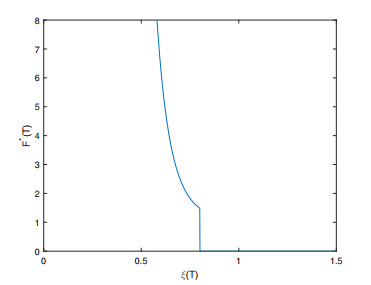
We consider the portfolio selection problem of maximizing a performance measure of the terminal wealth faced by a manager with a stochastic benchmark. We transform the non-linear fractional optimization problem into a non-fractional optimization problem based on the fractional programming method. When the penalty and reward functions are both power functions, the stochastic benchmark we consider allows us to derive the explicit form of the optimal investment strategy by combining the linearization method, the martingale method, the change of measure, and the concavification method. Theoretical and numerical results show that the optimal terminal relative performance ends up with zero from a certain value of the price density, which reflects the moral hazard problem.

References

[1]	H. M. Markowitz, Portfolio selection, J. Financ., 7 (1952), 77–91. https://doi.org/10.1111/j.1540-6261.1952.tb01525.x doi: 10.1111/j.1540-6261.1952.tb01525.x
[2]	D. Kahneman, A. Tversky, Prospect theory: An analysis of decision under risk, Econometrica, 47 (1979), 363–391. https://doi.org/10.2307/1914185 doi: 10.2307/1914185
[3]	A. Tversky, D. Kahneman, Advances in prospect theory: Cumulative representation of uncertainty, J. Risk Uncertainty, 5 (1992), 297–323. https://doi.org/10.1007/BF00122574 doi: 10.1007/BF00122574
[4]	A. B. Berkelaar, R. Kouwenberg, T. Post, Optimal portfolio choice under loss aversion, Rev. Econ. Stat., 86 (2004), 973–987. https://doi.org/10.1162/0034653043125167 doi: 10.1162/0034653043125167
[5]	G. H. Guan, Z. X. Liang, Y. Xia, Optimal management of DC pension fund under the relative performance ratio and VaR constraint, Eur. J. Oper. Res., 305 (2023), 868–886. https://doi.org/10.1016/j.ejor.2022.06.012 doi: 10.1016/j.ejor.2022.06.012
[6]	Z. Chen, Z. F. Li, Y. Zeng, Portfolio choice with illiquid asset for a loss-averse pension investor, Insur. Math. Econ., 108 (2023), 60–83. https://doi.org/10.1016/j.insmatheco.2022.10.003 doi: 10.1016/j.insmatheco.2022.10.003
[7]	H. Lin, D. Saunders, C. Weng, Optimal investment strategies for participating contracts, Insur. Math. Econ., 73 (2017), 137–155. https://doi.org/10.1016/j.insmatheco.2017.02.001 doi: 10.1016/j.insmatheco.2017.02.001
[8]	S. X. Wang, X. M. Rong, H. Zhao, Optimal investment and benefit payment strategy under loss aversion for target benefit pension plans, Appl. Math. Comput., 346 (2019), 205–218. https://doi.org/10.1016/j.amc.2018.10.030 doi: 10.1016/j.amc.2018.10.030
[9]	Y. H. Dong, H. Zheng, Optimal investment with S-shaped utility and trading and value at risk constraints: An application to defined contribution pension plan, Eur. J. Oper. Res., 281 (2020), 346–356. https://doi.org/10.1016/j.ejor.2019.08.034 doi: 10.1016/j.ejor.2019.08.034
[10]	J. N. Carpenter, Does option compensation increase managerial risk appetite? J. Finance, 55 (2000), 2311–2331. https://doi.org/10.1111/0022-1082.00288 doi: 10.1111/0022-1082.00288
[11]	T. Nguyen, M. Stadje, Nonconcave optimal investment with Value-at-Risk constraint: An application to life insurance contracts, SIAM J. Control Optim., 58 (2020), 895–936. https://doi.org/10.1137/18M1217322 doi: 10.1137/18M1217322
[12]	Y. H. Dong, H. Zheng, Optimal investment of DC pension plan under short-selling constraints and portfolio insurance, Insur. Math. Econ., 85 (2019), 47–59. https://doi.org/10.1016/j.insmatheco.2018.12.005 doi: 10.1016/j.insmatheco.2018.12.005
[13]	F. A. Sortino, L. N. Price, Performance measurement in a downside risk framework, J. Invest., 3 (1994), 59–64. https://doi.org/10.3905/joi.3.3.59 doi: 10.3905/joi.3.3.59
[14]	F. A. Sortino, R. Van Der Meer, A. Plantinga, The dutch triangle, J. Portfolio Manage., 26 (1999), 50–57. https://doi.org/10.3905/jpm.1999.319775 doi: 10.3905/jpm.1999.319775
[15]	P. D. Kaplan, J. A. Knowles, Kappa: A generalized downside risk-adjusted performance measure, J. Perform. Meas., 8 (2004), 42–54.
[16]	C. Keating, W. F. Shadwick, A universal performance measure, J. Perform. Meas., 6 (2002), 59–84.
[17]	C. Bernard, S. Vanduffel, J. Ye, Optimal strategies under Omega ratio, Eur. J. Oper. Res., 275 (2019), 755–767. https://doi.org/10.1016/j.ejor.2018.11.046 doi: 10.1016/j.ejor.2018.11.046
[18]	H. Lin, D. Saunders, C. Weng, Portfolio optimization with performance ratios, Int. J. Theor. Appl. Fin., 22 (2019), 1950022. https://doi.org/10.1142/S0219024919500225 doi: 10.1142/S0219024919500225
[19]	J. C. Cox, C. F. Huang, Optimal consumption and portfolio policies when asset prices follow a diffusion process, J. Econ. Theory, 49 (1989), 33–83. https://doi.org/10.1016/0022-0531(89)90067-7 doi: 10.1016/0022-0531(89)90067-7
[20]	I. Karatzas, S. E. Shreve, Brownian motion and stochastic calculus, New York: Springer, 1991. https://doi.org/10.1007/978-1-4612-0949-2
[21]	J. Cvitanic, I. Karatzas, Convex duality in constrained portfolio optimization, Ann. Appl. Probab., 2 (1992), 767–818. https://doi.org/10.1214/aoap/1177005576 doi: 10.1214/aoap/1177005576
[22]	I. Karatzas, J. P. Lehoczky, S. P. Sethi, S. E. Shreve, Explicit solution of a general consumption/investment problem, In: Stochastic optimization, 1986, 59–69. https://doi.org/10.1007/BFb0007083
[23]	S. Basak, A. Shapiro, L. Teplá, Risk management with benchmarking, Manage. Sci., 52 (2006), 542–557. https://doi.org/10.1287/mnsc.1050.0476 doi: 10.1287/mnsc.1050.0476
[24]	D. Zieling, A. Mahayni, S. Balder, Performance evaluation of optimized portfolio insurance strategies, J. Bank. Financ., 43 (2014), 212–225. https://doi.org/10.1016/j.jbankfin.2014.03.027 doi: 10.1016/j.jbankfin.2014.03.027
[25]	G. Guastaroba, R. Mansini, W. Ogryczak, M. G. Speranza, Linear programming models based on omega ratio for the enhanced index tracking problem, Eur. J. Oper. Res., 251 (2016), 938–956. https://doi.org/10.1016/j.ejor.2015.11.037 doi: 10.1016/j.ejor.2015.11.037
[26]	S. Kane, M. C. Bartholomew-Biggs, M. Cross, M. Dewar, Optimizing omega, J. Glob. Optim., 45 (2009), 153–167. https://doi.org/10.1007/s10898-008-9396-5 doi: 10.1007/s10898-008-9396-5
[27]	M. Nicolosi, Optimal strategy for a fund manager with option compensation, Decisions Econ. Finan., 41 (2018), 1–17. https://doi.org/10.1007/s10203-017-0204-x doi: 10.1007/s10203-017-0204-x
[28]	X. D. He, S. Kou, Profit sharing in hedge funds, Math. Financ., 28 (2018), 50–81. https://doi.org/10.1111/mafi.12143 doi: 10.1111/mafi.12143
[29]	H. Jin, Z. Q. Xu, X. Y. Zhou, A convex stochastic optimization problem arising from portfolio selection, Math. Financ., 18 (2008), 171–183. https://doi.org/10.1111/j.1467-9965.2007.00327.x doi: 10.1111/j.1467-9965.2007.00327.x
[30]	G. H. Guan, Z. X. Liang, Optimal management of DC pension plan under loss aversion and value-at-risk constraints, Insur. Math. Econ., 69 (2016), 224–237. https://doi.org/10.1016/j.insmatheco.2016.05.014 doi: 10.1016/j.insmatheco.2016.05.014
[31]	C. Reichlin, Utility maximization with a given pricing measure when the utility is not necessarily concave, Math. Financ. Econ., 7 (2013), 531–556. https://doi.org/10.1007/s11579-013-0093-x doi: 10.1007/s11579-013-0093-x

Reader Comments

Your name:*

Email:*
© 2025 the Author(s), licensee AIMS Press. This is an open access article distributed under the terms of the Creative Commons Attribution License (http://creativecommons.org/licenses/by/4.0)