Dynamics on semi-discrete Mackey-Glass model

Yulong Li; Long Zhou; Fengjie Geng; Yulong Li; Long Zhou; Fengjie Geng

doi:10.3934/math.2025130

AIMS Mathematics

2025, Volume 10, Issue 2: 2771-2807. doi: 10.3934/math.2025130

Previous Article Next Article

Research article

Dynamics on semi-discrete Mackey-Glass model

School of Science, China University of Geosciences (Beijing), 100083, Beijing, China

Received: 18 December 2024 Revised: 17 January 2025 Accepted: 06 February 2025 Published: 14 February 2025
MSC : 39A28, 39A30, 39A60

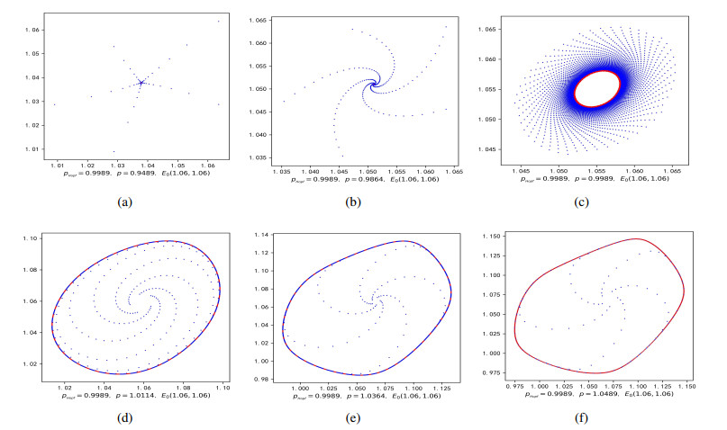
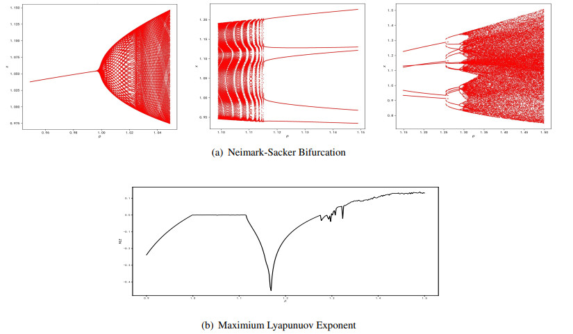
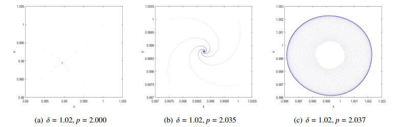
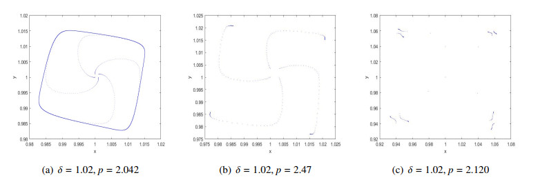
Red blood cells play an extremely important role in human metabolism, and the study of hematopoietic models is of great significance in biology and medicine. A kind of semi-discrete hetmatopoietic model named Mackey-Glass Model was proposed and analyzed in this paper. The existences, stabilities, and local dynamics of the fixed points were discussed. By using bifurcation theory, we studied the Neimark-Sacker bifurcation, saddle-node bifurcation, and strong resonance of 1:4. The numerical simulations were presented to illustrate the results of theoretical analysis obtained in this paper, and complex dynamical behaviors were found such as invariant cycles, heteroclinic cycles and Li-Yorke chaos. In addition, a new periodic bubbling phenomenon was discovered in numerical simulations. These not only reflect the richer dynamical behaviors of the semi-discrete models, but also some reflect the complex metabolic characteristics of the hematopoietic system under environmental intervention.
- semi-discrete hetmatopoietic model,
- Neimark-Sacker bifurcation,
- saddle-node bifurcation,
- strong resonance of 1:4,
- numerical simulations
Citation: Yulong Li, Long Zhou, Fengjie Geng. Dynamics on semi-discrete Mackey-Glass model[J]. AIMS Mathematics, 2025, 10(2): 2771-2807. doi: 10.3934/math.2025130

Related Papers:

Abstract

Red blood cells play an extremely important role in human metabolism, and the study of hematopoietic models is of great significance in biology and medicine. A kind of semi-discrete hetmatopoietic model named Mackey-Glass Model was proposed and analyzed in this paper. The existences, stabilities, and local dynamics of the fixed points were discussed. By using bifurcation theory, we studied the Neimark-Sacker bifurcation, saddle-node bifurcation, and strong resonance of 1:4. The numerical simulations were presented to illustrate the results of theoretical analysis obtained in this paper, and complex dynamical behaviors were found such as invariant cycles, heteroclinic cycles and Li-Yorke chaos. In addition, a new periodic bubbling phenomenon was discovered in numerical simulations. These not only reflect the richer dynamical behaviors of the semi-discrete models, but also some reflect the complex metabolic characteristics of the hematopoietic system under environmental intervention.

References

[1]	A. Beuter, L. Glass, M. C. Mackey, M. S. Titcombe, Nonlinear dynamics in physiology and medicine, Springer, 2003. http://dx.doi.org/10.1007/978-0-387-21640-9
[2]	A. Fahsi, M. Belhaq, Analytical approximation of heteroclinic bifurcation in a 1:4 resonance, Int. J. Bifurc. Chaos, 22 (2012), 1250294. http://dx.doi.org/10.1142/S021812741250294X doi: 10.1142/S021812741250294X
[3]	A. Wan, J. Wei, Bifurcation analysis of Mackey-Glass electronic circuits model with delayed feedback, Nonlinear Dynam., 57 (2009), 85–96. http://dx.doi.org/10.1007/s11071-008-9422-7 doi: 10.1007/s11071-008-9422-7
[4]	A. Zaghrout, A. Mmar, A. EI-Sheikh, Oscillations and global attractivity in delay differential equations of population dynamics, Appl. Math. Comput., 77 (1996), 195–204. http://dx.doi.org/10.1016/S0096-3003(95)00213-8 doi: 10.1016/S0096-3003(95)00213-8
[5]	B. Krauskopf, Bifurcations at $\infty$ in a model for 1:4 resonance, Ergod. Theory Dyn. Syst., 17 (1997), 899–931. http://dx.doi.org/10.1017/s0143385797085039 doi: 10.1017/s0143385797085039
[6]	B. Li, Z. He, 1:2 and 1:4 resonances in a two-dimensional discrete Hindmarsh-Rose model, Nonlinear Dyn., 79 (2015), 705–720. http://dx.doi.org/10.1007/s11071-014-1696-3 doi: 10.1007/s11071-014-1696-3
[7]	C. Bonatto, J. A. C. Gallas, Periodicity hub and nested spirals in the phase diagram of a simple resistive circuit, Phys. Rev. Lett., 101 (2008), 054101. http://dx.doi.org/10.1103/physrevlett.101.054101 doi: 10.1103/physrevlett.101.054101
[8]	C. Wang, X. Li, Further investigations into the stability and bifurcation of a discrete predator-prey model, J. Math. Anal. Appl., 422 (2015), 920–939. http://dx.doi.org/10.1016/j.jmaa.2014.08.058 doi: 10.1016/j.jmaa.2014.08.058
[9]	C. Wang, X. Li, Stability and Neimark-Sacker bifurcation of a semi-discrete population model, J Appl. Anal. Comput., 4 (2014), 419–435. http://dx.doi.org/10.11948/2014024 doi: 10.11948/2014024
[10]	D. Mukherjee, Dynamics of A discrete-time ecogenetic predator-prey model, Commun. Biomath. Sci., 5 (2023), 161–169. http://dx.doi.org/10.5614/cbms.2022.5.2.5 doi: 10.5614/cbms.2022.5.2.5
[11]	D. Wu, H. Zhao, Complex dynamics of a discrete predator-prey model with the prey subject to the Allee effect, J. Differ. Equ. Appl., 23 (2017), 1765–1806. http://dx.doi.org/10.1080/10236198.2017.1367389 doi: 10.1080/10236198.2017.1367389
[12]	E. Shahverdiev, R. A. Nuriev, L. H. Hashimova, E. M. Huseynova, R. H. Hashimov, Chaos synchronization in the multifeedback Mackey-Glass model, Int. J. Mod. Phys. B, 19 (2005), 3613–3618. http://dx.doi.org/10.1142/S0217979205032346 doi: 10.1142/S0217979205032346
[13]	I. Tamas, S. Gabor, Semi-discretization method for delayed systems, Int. J. Numer. Meth. Eng., 55 (2002), 503–518. http://dx.doi.org/10.1002/nme.505 doi: 10.1002/nme.505
[14]	J. G. Freire, J. A. C. Gallas, Cyclic organization of stable periodic and chaotic pulsations in Hartleys oscillator, Chaos Soliton. Fract., 59 (2014), 129–134. https://doi.org/10.1016/j.chaos.2013.12.007 doi: 10.1016/j.chaos.2013.12.007
[15]	J. Guckenheimer, Multiple bifurcation problems of codimension two, SIAM J. Math. Anal., 15 (1984), 1–49. http://dx.doi.org/10.1137/0515001 doi: 10.1137/0515001
[16]	J. Vandermeer, Period bubbling in simple ecological models: Pattern and chaos formation in a quartic model, Ecol. Model., 95 (1997), 311–317. https://doi.org/10.1016/S0304-3800(96)00046-4 doi: 10.1016/S0304-3800(96)00046-4
[17]	K. Gopalsamy, M. Kulenović, G. Ladas, Oscillations and global attractivity in models of hematopoiesis, J. Dyn. Differ. Equ., 2 (1990), 117–132. http://dx.doi.org/10.1007/BF01057415 doi: 10.1007/BF01057415
[18]	K. J. Hale, N. Sternberg, Onset of chaos in differential delay equations, J. Comput. Phys., 77 (1988), 221–239. https://doi.org/10.1016/0021-9991(88)90164-7 doi: 10.1016/0021-9991(88)90164-7
[19]	L. Cheng, H. Cao, Bifurcation analysis of a discrete-time ratio-dependent predator-prey model with Allee Effect, Commun. Nonlinear Sci., 38 (2016), 288–302. https://doi.org/10.1016/j.cnsns.2016.02.038 doi: 10.1016/j.cnsns.2016.02.038
[20]	L. Lv, X. Li, Stability and bifurcation analysis in a discrete predator-prey system of Leslie type with radio-dependent simplified Holling Type Ⅳ functionalresponse, Mathematics, 12 (2024), 1803. http://dx.doi.org/10.3390/math12121803 doi: 10.3390/math12121803
[21]	M. B. Almatrafia, M. Berkal, Stability and bifurcation analysis of predator-prey model with Allee effect using conformable derivatives, J. Math. Comput. Sci., 36 (2025), 299–316. http://dx.doi.org/10.22436/jmcs.036.03.05 doi: 10.22436/jmcs.036.03.05
[22]	M. Berkal, M. B. Almatrafi, Bifurcation and stability of two-dimensional activator-inhibitor model with fractional-order derivative, Fractal Fract., 7 (2023), 1–18. http://dx.doi.org/10.3390/fractalfract7050344 doi: 10.3390/fractalfract7050344
[23]	M. S. Peng, Multiple bifurcations and periodic "bubbling" in a delay population model, Chaos Soliton. Fract., 25(2005), 1123–1130. https://doi.org/10.1016/j.chaos.2004.11.087 doi: 10.1016/j.chaos.2004.11.087
[24]	M. Wazewsa, A. Lasota, Mathematical problems of the dynamics of a system of red blood cells, Math. Stosowana, 6 (1976), 23–40. http://dx.doi.org/10.14708/ma.v4i6.1173 doi: 10.14708/ma.v4i6.1173
[25]	M. Zhao, Y. Du, Stability and bifurcation analysis of an amensalism system with allee effect, Adv. Differ. Equ., 1 (2020), 1–13. http://dx.doi.org/10.1186/s13662-020-02804-9 doi: 10.1186/s13662-020-02804-9
[26]	M. Zhao, C. Li, J. Wang, Complex dynamic behaviors of a discrete-time predator-prey system, J. Appl. Anal. Comput., 7 (2017), 478–500. http://dx.doi.org/10.11948/2017030 doi: 10.11948/2017030
[27]	N. Yi, Q. L. Zhang, P. Liu, Y. P. Lin, Codimension-two bifurcations analysis and tracking control on a discrete epidemic model, J. Syst. Sci. Complex., 24 (2011), 1033–1056. http://dx.doi.org/10.1007/s11424-011-9041-0 doi: 10.1007/s11424-011-9041-0
[28]	P. Amil, C. Cabeza, C. Masoller, A. C. Martí, Organization and identification of solutions in the time-delayed Mackey-Glass model, Chaos Interd. J. Nonlinear Sci., 25 (2015), 035202–035204. http://dx.doi.org/10.1063/1.4918593 doi: 10.1063/1.4918593
[29]	P. Amil, C. Cabeza, A. C. Marti, Exact discrete-time implementation of the Mackey-Glass delayed model, IEEE T. Circuits-II, 62 (2015), 681–685. http://dx.doi.org/10.1109/TCSII.2015.2415651 doi: 10.1109/TCSII.2015.2415651
[30]	Q. L. Chen, Z. D. Teng, L. Wang, H. Jiang, The existence of codimension-two bifurcation in a discrete SIS epidemic model with standard incidence, Nonlinear Dyn. 71 (2013), 55–73. http://dx.doi.org/10.1007/s11071-012-0641-6 doi: 10.1007/s11071-012-0641-6
[31]	R. Ma, Y. Bai, F. Wang, Dynamical behavior of a two-dimensional discrete predator-prey model with prey refuse and fear factor, J. Appl. Anal. Comput., 10 (2020), 1683–1697. http://dx.doi.org/10.11948/20190426 doi: 10.11948/20190426
[32]	S. Akhtar, R. Ahmed, M. Batool, N. A. Shah, J. D. Chung, Stability, bifurcation and chaos control of a discretized Leslie prey-predator model, Chaos Soliton. Fract., 152 (2021), 1–10. https://doi.org/10.1016/j.chaos.2021.111345 doi: 10.1016/j.chaos.2021.111345
[33]	S. G. Ruan, D. M. Xiao, Global analysis in a predator-prey system with nonmonotonic functional response, SIAM J. Appl. Math., 61 (2001), 1445–1472. http://dx.doi.org/10.1137/S0036139999361896 doi: 10.1137/S0036139999361896
[34]	S. S. Rana, Bifurcations and chaos control in a discrete-time predator-prey system of Leslie type, J. Appl. Anal. Comput., 9 (2019), 31–44. http://dx.doi.org/10.11948/2019.31 doi: 10.11948/2019.31
[35]	S. S. Rana, M. Uddin, Dynamics of a discrete-time chaotic lü system, Pan-Am. J. Math., 1 (2022), 1–7. http://dx.doi.org/10.28919/cpr-pajm/1-7 doi: 10.28919/cpr-pajm/1-7
[36]	S. L. Badjate, S. V. Dudul, Prediction of Mackey-Glass chaotic time series with effect of superimposed noise using FTLRNN model, New York, 2008. Available from: https://api.semanticscholar.org/CorpusID: 59747728.
[37]	T. Y. Li, J. A. Yorke, Period three implies chaos, Am. Math. Mon., 82 (1975), 985–992. Available from: https://www.jstor.org/stable/2318254.
[38]	W. Cheng, X. Li, Stability and Neimark-Sacker bifurcation of a semi-discrete population model, J. Appl. Anal. Comput., 4 (2014), 419–435. http://dx.doi.org/10.11948/2014024 doi: 10.11948/2014024
[39]	W. Li, X. Li, Neimark-Sacker bifurcation of a semi-discrete hematopoiesis model, J. Appl. Anal. Comput., 8 (2018), 1679–1693. http://dx.doi.org/10.11948/2018.1679 doi: 10.11948/2018.1679
[40]	W. Yao, X. Li, Bifurcation difference induced by different discrete methods in a discrete predator-prey model, J. Nonlinear Model. Anal., 4 (2022), 64–79. http://dx.doi.org/10.12150/jnma.2022.64 doi: 10.12150/jnma.2022.64
[41]	X. Jin, X. Li, Dynamics of a discrete two-species competitive model with Michaelis-Menten type harvesting in the first species, J. Nonlinear Model. Anal., 5 (2023), 494–523. http://dx.doi.org/10.12150/jnma.2023.494 doi: 10.12150/jnma.2023.494
[42]	X. L. Liu, D. M. Xiao, Complex dynamic behaviors of a discrete-time predator-prey system, Chaos Soliton. Fract., 32 (2007), 80–94. https://doi.org/10.1016/j.chaos.2005.10.081 doi: 10.1016/j.chaos.2005.10.081
[43]	X. L. Liu, S. Q. Liu, Codimension-two bifurcations analysis in two-dimensional Hindmarsh-Rose model, Nonlinear Dyn., 67 (2012), 847–857. http://dx.doi.org/10.1007/s11071-011-0030-6 doi: 10.1007/s11071-011-0030-6
[44]	Y. A. Kuznetsov, Elements of applied bifurcation theory, 4 Eds., Springer, 2023. http://dx.doi.org/10.1007/978-3-031-22007-4
[45]	Y. A. Kuznetsov, H. Meijer, Numerical normal forms for codim 2 bifurcations of fixed points with at most two critical eigenvalues, SIAM J. Sci. Comput., 26 (2005), 1932–1954. http://dx.doi.org/10.1137/030601508 doi: 10.1137/030601508
[46]	Y. L. Li, D. M. Xiao, Bifurcations of a predator-prey system of Holling and Leslie types, Chaos Soliton. Fract., 34 (2007), 606–620. https://doi.org/10.1016/j.chaos.2006.03.068 doi: 10.1016/j.chaos.2006.03.068
[47]	Y. Hong, Global dynamics of a diffusive phytoplankton-zooplankton model with toxic substances effect and delay, Math. Biosci. Eng., 19 (2022), 6712–6730. https://doi.org/10.3934/mbe.2022316 doi: 10.3934/mbe.2022316
[48]	Y. Li, H. Cao, Bifurcation and comparison of a discrete-time Hindmarsh-Rose model, J. Appl. Anal. Comput., 13 (2023), 34–56. http://dx.doi.org/10.11948/20210204 doi: 10.11948/20210204
[49]	Z. Jing, J. Yang, Bifurcation and chaos in discrete-time predator–prey system, Chaos Soliton. Fract., 27 (2006), 259–277. https://doi.org/10.1016/j.chaos.2005.03.040 doi: 10.1016/j.chaos.2005.03.040
[50]	Z. Wei, Y. Xia, T. Zhang, Stability and bifurcation analysis of an amensalism model with weak allee effect, Qual. Theor. Dyn. Syst., 19 (2020), 1–15. https://doi.org/10.1007/s12346-020-00341-0 doi: 10.1007/s12346-020-00341-0

Reader Comments

Your name:*

Email:*
© 2025 the Author(s), licensee AIMS Press. This is an open access article distributed under the terms of the Creative Commons Attribution License (http://creativecommons.org/licenses/by/4.0)