Stability, bifurcation, and chaos control in a discrete predator-prey model with strong Allee effect

Ali Al Khabyah; Rizwan Ahmed; Muhammad Saeed Akram; Shehraz Akhtar; Ali Al Khabyah; Rizwan Ahmed; Muhammad Saeed Akram; Shehraz Akhtar

doi:10.3934/math.2023408

AIMS Mathematics

2023, Volume 8, Issue 4: 8060-8081. doi: 10.3934/math.2023408

Previous Article Next Article

Research article

Stability, bifurcation, and chaos control in a discrete predator-prey model with strong Allee effect

1.
Department of Mathematics, College of Science, Jazan University, New Campus, Saudi Arabia
2.
Department of Mathematics, Air University Multan Campus, Multan, Pakistan
3.
Department of Mathematics, Faculty of Science, Ghazi University, Dera Ghazi Khan, Pakistan
4.
Department of Mathematics, The Islamia University of Bahawalpur Rahim Yar Khan Campus, Rahim Yar Khan, Pakistan

Received: 19 October 2022 Revised: 11 January 2023 Accepted: 16 January 2023 Published: 31 January 2023
MSC : 39A28, 39A30

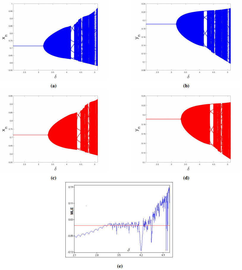
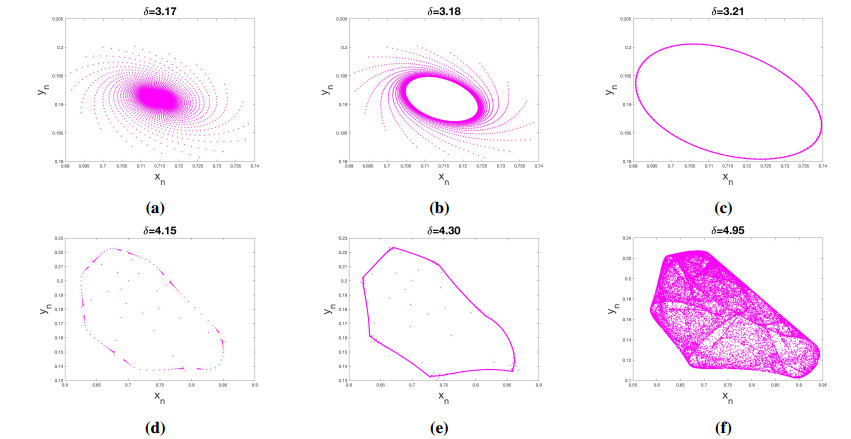
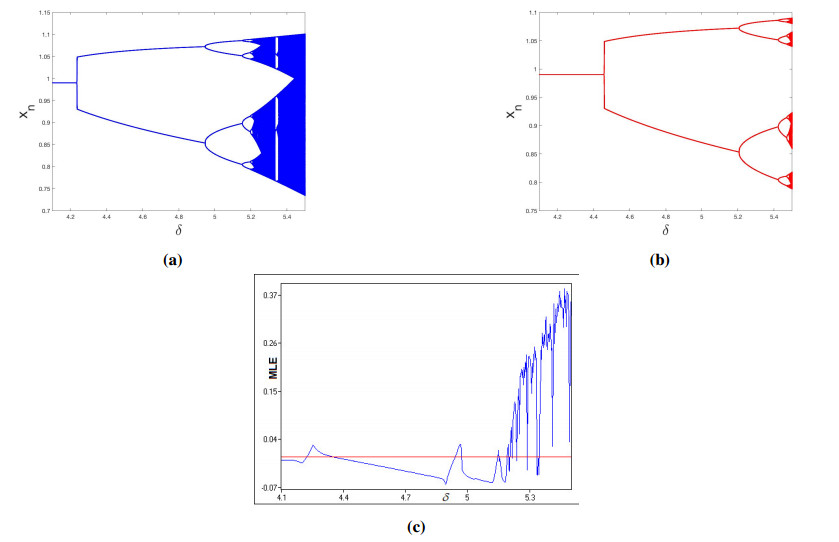
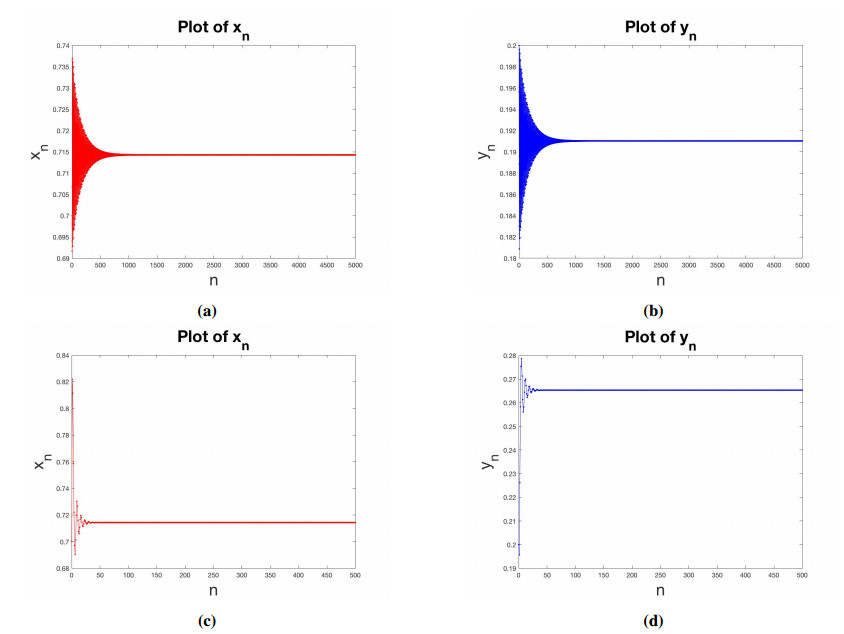
This work considers a discrete-time predator-prey system with a strong Allee effect. The existence and topological classification of the system's possible fixed points are investigated. Furthermore, the existence and direction of period-doubling and Neimark-Sacker bifurcations are explored at the interior fixed point using bifurcation theory and the center manifold theorem. A hybrid control method is used for controlling chaos and bifurcations. Some numerical examples are presented to verify our theoretical findings. Numerical simulations reveal that the discrete model has complex dynamics. Moreover, it is shown that the system with the Allee effect requires a much longer time to reach its interior fixed point.
- predator-prey,
- Holling type-Ⅱ,
- Allee effect,
- stability,
- bifurcation
Citation: Ali Al Khabyah, Rizwan Ahmed, Muhammad Saeed Akram, Shehraz Akhtar. Stability, bifurcation, and chaos control in a discrete predator-prey model with strong Allee effect[J]. AIMS Mathematics, 2023, 8(4): 8060-8081. doi: 10.3934/math.2023408

Related Papers:

Abstract

This work considers a discrete-time predator-prey system with a strong Allee effect. The existence and topological classification of the system's possible fixed points are investigated. Furthermore, the existence and direction of period-doubling and Neimark-Sacker bifurcations are explored at the interior fixed point using bifurcation theory and the center manifold theorem. A hybrid control method is used for controlling chaos and bifurcations. Some numerical examples are presented to verify our theoretical findings. Numerical simulations reveal that the discrete model has complex dynamics. Moreover, it is shown that the system with the Allee effect requires a much longer time to reach its interior fixed point.

References

[1]	A. J. Lotka, Elements of physical biology, Williams & Wilkins, 1925.
[2]	V. Volterra, Variazioni e fluttuazioni del numero d'individui in specie animali conviventi, Società anonima tipografica "Leonardo da Vinci", 1927.
[3]	S. Pal, N. Pal, S. Samanta, J. Chattopadhyay, Effect of hunting cooperation and fear in a predator-prey model, Ecol. Complex., 39 (2019), 100770. https://doi.org/10.1016/j.ecocom.2019.100770 doi: 10.1016/j.ecocom.2019.100770
[4]	S. Kumar, H. Kharbanda, Chaotic behavior of predator-prey model with group defense and non-linear harvesting in prey, Chaos Solitons Fract., 119 (2019), 19–28. https://doi.org/10.1016/j.chaos.2018.12.011 doi: 10.1016/j.chaos.2018.12.011
[5]	Y. Zhou, W. Sun, Y. F. Song, Z. G. Zheng, J. H. Lu, S. H. Chen, Hopf bifurcation analysis of a predator-prey model with Holling-Ⅱ type functional response and a prey refuge, Nonlinear Dyn., 97 (2019), 1439–1450. 10.1007/s11071-019-05063-w doi: 10.1007/s11071-019-05063-w
[6]	S. Akhtar, R. Ahmed, M. Batool, N. A. Shah, J. D. Chung, Stability, bifurcation and chaos control of a discretized Leslie prey-predator model, Chaos Solitons Fract., 152 (2021), 111345. https://doi.org/10.1016/j.chaos.2021.111345 doi: 10.1016/j.chaos.2021.111345
[7]	H. Deng, F. D. Chen, Z. L. Zhu, Z. Li, Dynamic behaviors of Lotka-Volterra predator-prey model incorporating predator cannibalism, Adv. Differ. Equ., 2019 (2019), 1–17. https://doi.org/10.1186/s13662-019-2289-8 doi: 10.1186/s13662-019-2289-8
[8]	C. S. Holling, Some characteristics of simple types of predation and parasitism, Can. Entomol., 91 (1959), 385–398. https://doi.org/10.4039/Ent91385-7 doi: 10.4039/Ent91385-7
[9]	P. H. Crowley, E. K. Martin, Functional responses and interference within and between year classes of a dragonfly population, J. N. Amer. Benthol. Soc., 8 (1989), 211–221. https://doi.org/10.2307/1467324 doi: 10.2307/1467324
[10]	J. R. Beddington, Mutual interference between parasites or predators and its effect on searching efficiency, J. Anim. Ecol., 44 (1975), 331–340. https://doi.org/10.2307/3866 doi: 10.2307/3866
[11]	D. L. DeAngelis, R. A. Goldstein, R. V. O'Neill, A model for tropic interaction, Ecology, 56 (1975), 881–892. https://doi.org/10.2307/1936298 doi: 10.2307/1936298
[12]	M. F. Elettreby, A. Khawagi, T. Nabil, Dynamics of a discrete prey-predator model with mixed functional response, Int. J. Bifurcat. Chaos, 29 (2019), 1950199. https://doi.org/10.1142/s0218127419501992 doi: 10.1142/s0218127419501992
[13]	S. M. Sohel Rana, U. Kulsum, Bifurcation analysis and chaos control in a discrete-time predator-prey system of Leslie type with simplified Holling type Ⅳ functional response, Discrete Dyn. Nat. Soc., 2017 (2017), 1–11. https://doi.org/10.1155/2017/9705985 doi: 10.1155/2017/9705985
[14]	C. Arancibia-Ibarra, P. Aguirre, J. Flores, P. van Heijster, Bifurcation analysis of a predator-prey model with predator intraspecific interactions and ratio-dependent functional response, Appl. Math. Comput., 402 (2021), 126152. https://doi.org/10.1016/j.amc.2021.126152 doi: 10.1016/j.amc.2021.126152
[15]	X. F. Chen, X. Zhang, Dynamics of the predator-prey model with the Sigmoid functional response, Stud. Appl. Math., 147 (2021), 300–318. https://doi.org/10.1111/sapm.12382 doi: 10.1111/sapm.12382
[16]	P. Panja, Combine effects of square root functional response and prey refuge on predator-prey dynamics, Int. J. Model. Simul., 41 (2021), 426–433. https://doi.org/10.1080/02286203.2020.1772615 doi: 10.1080/02286203.2020.1772615
[17]	H. J. Alsakaji, S. Kundu, F. A. Rihan, Delay differential model of one-predator two-prey system with Monod-Haldane and Holling type Ⅱ functional responses, Appl. Math. Comput., 397 (2021), 125919. https://doi.org/10.1016/j.amc.2020.125919 doi: 10.1016/j.amc.2020.125919
[18]	W. C. Allee, Animal aggregations: a study in general sociology, Chicago: University of Chicago Press, 1931. https://doi.org/10.5962/bhl.title.7313
[19]	M. H. Wang, M. Kot, Speeds of invasion in a model with strong or weak Allee effects, Math. Biosci., 171 (2001), 83–97. https://doi.org/10.1016/s0025-5564(01)00048-7 doi: 10.1016/s0025-5564(01)00048-7
[20]	S. Vinoth, R. Sivasamy, K. Sathiyanathan, B. Unyong, G. Rajchakit, R. Vadivel, et al., The dynamics of a Leslie type predator-prey model with fear and Allee effect, Adv. Differ. Equ., 2021 (2021), 1–22. https://doi.org/10.1186/s13662-021-03490-x doi: 10.1186/s13662-021-03490-x
[21]	Y. F. Du, B. Niu, J. J. Wei, Dynamics in a predator-prey model with cooperative hunting and Allee effect, Mathematics, 9 (2021), 1–40. https://doi.org/10.3390/math9243193 doi: 10.3390/math9243193
[22]	H. Molla, S. Sarwardi, S. R. Smith, M. Haque, Dynamics of adding variable prey refuge and an Allee effect to a predator-prey model, Alex. Eng. J., 61 (2022), 4175–4188. https://doi.org/10.1016/j.aej.2021.09.039 doi: 10.1016/j.aej.2021.09.039
[23]	Z. C. Shang, Y. H. Qiao, Bifurcation analysis of a Leslie-type predator-prey system with simplified Holling type Ⅳ functional response and strong Allee effect on prey, Nonlinear Anal. Real World Appl., 64 (2022), 103453. https://doi.org/10.1016/j.nonrwa.2021.103453 doi: 10.1016/j.nonrwa.2021.103453
[24]	K. Fang, Z. L. Zhu, F. D. Chen, Z. Li, Qualitative and bifurcation analysis in a Leslie-Gower model with Allee effect, Qual. Theory Dyn. Syst., 21 (2022), 1–19. https://doi.org/10.1007/s12346-022-00591-0 doi: 10.1007/s12346-022-00591-0
[25]	Y. N. Zeng, P. Yu, Complex dynamics of predator-prey systems with Allee effect, Int. J. Bifurcat. Chaos, 32 (2022), 2250203. https://doi.org/10.1142/s0218127422502030 doi: 10.1142/s0218127422502030
[26]	Y. D. Ma, M. Zhao, Y. F. Du, Impact of the strong Allee effect in a predator-prey model, AIMS Math., 7 (2022), 16296–16314. https://doi.org/10.3934/math.2022890 doi: 10.3934/math.2022890
[27]	M. J. Khanghahi, R. K. Ghaziani, Bifurcation analysis of a modified May-Holling-Tanner predator-prey model with Allee effect, Bull. Iran. Math. Soc., 48 (2022), 3405–3437. https://doi.org/10.1007/s41980-022-00698-9 doi: 10.1007/s41980-022-00698-9
[28]	J. Ye, Y. Wang, Z. Jin, C. J. Dai, M. Zhao, Dynamics of a predator-prey model with strong Allee effect and nonconstant mortality rate, Math. Biosci. Eng., 19 (2022), 3402–3426. https://doi.org/10.3934/mbe.2022157 doi: 10.3934/mbe.2022157
[29]	L. Y. Lai, Z. L. Zhu, F. D. Chen, Stability and bifurcation in a predator-prey model with the additive Allee effect and the fear effect, Mathematics, 8 (2020), 1–21. https://doi.org/10.3390/math8081280 doi: 10.3390/math8081280
[30]	M. Zhao, C. P. Li, J. L. Wang, Complex dynamic behaviors of a discrete-time predator-prey system, J. Appl. Anal. Comput., 7 (2017), 478–500. https://doi.org/10.11948/2017030 doi: 10.11948/2017030
[31]	P. Baydemir, H. Merdan, E. Karaoglu, G. Sucu, Complex dynamics of a discrete-time prey-predator system with Leslie type: stability, bifurcation analyses and chaos, Int. J. Bifurcat. Chaos, 30 (2020), 2050149. https://doi.org/10.1142/s0218127420501497 doi: 10.1142/s0218127420501497
[32]	S. M. Sohel Rana, Dynamics and chaos control in a discrete-time ratio-dependent Holling-Tanner model, J. Egypt. Math. Soc., 27 (2019), 1–16. https://doi.org/10.1186/s42787-019-0055-4 doi: 10.1186/s42787-019-0055-4
[33]	P. A. Naik, Z. Eskandari, M. Yavuz, J. Zu, Complex dynamics of a discrete-time Bazykin-Berezovskaya prey-predator model with a strong Allee effect, J. Comput. Appl. Math., 413 (2022), 114401. https://doi.org/10.1016/j.cam.2022.114401 doi: 10.1016/j.cam.2022.114401
[34]	A. C. Luo, Regularity and complexity in dynamical systems, New York: Springer, 2012.
[35]	X. S. Luo, G. R. Chen, B. H. Wang, J. Q. Fang, Hybrid control of period-doubling bifurcation and chaos in discrete nonlinear dynamical systems, Chaos Solitons Fract., 18 (2003), 775–783. https://doi.org/10.1016/s0960-0779(03)00028-6 doi: 10.1016/s0960-0779(03)00028-6

Reader Comments

Your name:*

Email:*
© 2023 the Author(s), licensee AIMS Press. This is an open access article distributed under the terms of the Creative Commons Attribution License (http://creativecommons.org/licenses/by/4.0)