Constructing boundary layer approximations in rotating magnetohydrodynamic fluids within cylindrical domains

Guanglei Zhang; Kexue Chen; Yifei Jia; Guanglei Zhang; Kexue Chen; Yifei Jia

doi:10.3934/math.2025128

AIMS Mathematics

2025, Volume 10, Issue 2: 2724-2749. doi: 10.3934/math.2025128

Previous Article Next Article

Research article Topical Sections

Constructing boundary layer approximations in rotating magnetohydrodynamic fluids within cylindrical domains

1.
Department of Mathematics, Jinan University, Guangzhou, China
2.
College of Mathematics and System Science, Xinjiang University, Urumqi, China

Received: 28 November 2024 Revised: 13 January 2025 Accepted: 23 January 2025 Published: 14 February 2025
MSC : 76D10, 76U05

This paper aims to investigate the effects of the Ekman-Hartmann boundary layer on rotating magnetohydrodynamics (MHD) within cylindrical domains, focusing on constructing approximate solutions within the boundary layer. We employed the multiscale analysis method to derive the approximate solutions, emphasizing the solutions at the cylinder's corners and lateral boundaries. Furthermore, we rigorously examined the asymptotic behavior of the rotating MHD flow in the limit case, proving its convergence to a two-dimensional damped and rotating dynamical system. These findings revealed the significant impact of high-speed rotation and strong magnetic fields on the structure and flow characteristics of the boundary layer, providing new insights into the dynamics of rotating MHD flows.
- magnetohydrodynamics,
- rotating dynamical system,
- Ekman-Hartmann boundary layer,
- cylinder domain,
- asymptotic behavior
Citation: Guanglei Zhang, Kexue Chen, Yifei Jia. Constructing boundary layer approximations in rotating magnetohydrodynamic fluids within cylindrical domains[J]. AIMS Mathematics, 2025, 10(2): 2724-2749. doi: 10.3934/math.2025128

Related Papers:

Abstract

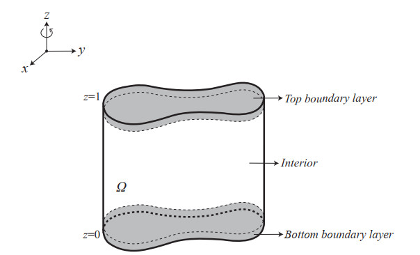
This paper aims to investigate the effects of the Ekman-Hartmann boundary layer on rotating magnetohydrodynamics (MHD) within cylindrical domains, focusing on constructing approximate solutions within the boundary layer. We employed the multiscale analysis method to derive the approximate solutions, emphasizing the solutions at the cylinder's corners and lateral boundaries. Furthermore, we rigorously examined the asymptotic behavior of the rotating MHD flow in the limit case, proving its convergence to a two-dimensional damped and rotating dynamical system. These findings revealed the significant impact of high-speed rotation and strong magnetic fields on the structure and flow characteristics of the boundary layer, providing new insights into the dynamics of rotating MHD flows.

References

[1]	L. Ali, P. Kumar, H. Poonia, S. Areekara, R. Apsari, The significant role of Darcy-Forchheimer and thermal radiation on Casson fluid flow subject to stretching surface: a case study of dusty fluid, Mod. Phys. Lett. B, 38 (2024), 2350215. http://doi.org/10.1142/S0217984923502159 doi: 10.1142/S0217984923502159
[2]	L. Ali, R. Apsari, A. Abbas, P. Tak, Entropy generation on the dynamics of volume fraction of nano-particles and coriolis force impacts on mixed convective nanofluid flow with significant magnetic effect, Numer. Heat Tr. A Appl., 2024 (2024), 1–16. https://doi.org/10.1080/10407782.2024.2360652 doi: 10.1080/10407782.2024.2360652
[3]	D. Bresch, B. Desjardins, D. Gérard-Varet, Rotating fluids in a cylinder, Discrete Cont. Dyn. Syst., 11 (2004), 47–82. http://doi.org/10.3934/dcds.2004.11.47 doi: 10.3934/dcds.2004.11.47
[4]	S. Chandrasekhar, Hydrodynamic and hydromagnetic stability, International Series of Monographs on Physics, 1961.
[5]	J. Y. Chemin, B. Desjardins, I. Gallagher, E. Grenier, Mathematical geophysics. An introduction to rotating fluids and the Navier-Stokes equations, Oxford University Press, 2006.
[6]	B. Desjardins, E. Dormy, E. Grenier, Stability of mixed Ekman-Hartmann boundary layers, Nonlinearity, 12 (1999), 181–199. http://doi.org/10.1088/0951-7715/12/2/001 doi: 10.1088/0951-7715/12/2/001
[7]	E. Dormy, Modélisation numérique de la dynamo terrestre, Paris: Institut de Physique du Globe de Paris, 1997.
[8]	E. Dormy, P. Cardin, D. Jault, MHD flow in a slightly differentially rotating spherical shell, with conducting inner core, in a dipolar magnetic field, Earth Planet. Sc. Lett., 160 (1998), 15–30. http://doi.org/10.1016/S0012-821X(98)00078-8 doi: 10.1016/S0012-821X(98)00078-8
[9]	G. Duvaut, J. L. Lions, Inéquations en thermoélasticité et magnétohydrodynamique, Arch. Rational Mech. Anal., 46 (1972), 241–279. https://doi.org/10.1007/BF00250512 doi: 10.1007/BF00250512
[10]	M. A. Fahmy, M. O. Alsulami, A. E. Abouelregal, Sensitivity analysis and design optimization of 3T rotating thermoelastic structures using IGBEM, AIMS Math., 7 (2022), 19902–19921. http://doi.org/10.3934/math.20221090 doi: 10.3934/math.20221090
[11]	M. A. Fahmy, A nonlinear fractional BEM model for magneto-thermo-visco-elastic ultrasound waves in temperature-dependent FGA rotating granular plates, Fractal Fract., 7 (2023), 214. http://doi.org/10.3390/fractalfract7030214 doi: 10.3390/fractalfract7030214
[12]	G. P. Galdi, An introduction to the mathematical theory of the Navier-Stokes equations, Springer Tracts in Natural Philosophy, 1994.
[13]	D. Gérard-Varet, A geometric optics type approach to fluid boundary layers, Commun. Part. Diff. Eq., 28 (2003), 1605–1626. https://doi.org/10.1081/PDE-120024524 doi: 10.1081/PDE-120024524
[14]	H. P. Greenspan, The theory of rotating fluids, Cambridge University Press, 1969.
[15]	J. Pedlosky, Geophysical fluid dynamics, New York: Springer-Verlag, 1979.
[16]	F. Rousset, Large mixed Ekman-Hartmann boundary layers in magnetohydrodynamics, Nonlinearity, 17 (2004), 503–518. http://doi.org/10.1088/0951-7715/17/2/008 doi: 10.1088/0951-7715/17/2/008
[17]	F. Rousset, Stability of large amplitude Ekman-Hartmann boundary layers in MHD: the case of ill-prepared data, Commun. Math. Phys., 259 (2005), 223–256. https://doi.org/10.1007/s00220-005-1371-0 doi: 10.1007/s00220-005-1371-0
[18]	F. Rousset, Asymptotic behavior of geophysical fluids in highly rotating balls, Z. Angew. Math. Phys., 58 (2007), 53–67. https://doi.org/10.1007/s00033-006-5021-y doi: 10.1007/s00033-006-5021-y
[19]	M. Sermange, R. Temam, Some mathematical questions related to the MHD equations, Commun. Pur. Appl. Math., 36 (1983), 635–664. https://doi.org/10.1002/cpa.3160360506 doi: 10.1002/cpa.3160360506
[20]	M. E. Schonbek, T. P. Schonbek, E. Süli, Large-time behaviour of solutions to the magnetohydrodynamics equations, Math. Ann., 304 (1996), 717–757. https://doi.org/10.1007/BF01446316 doi: 10.1007/BF01446316
[21]	S. Ukai, The incompressible limit and the initial layer of the compressible Euler equation, J. Math. Kyoto Univ., 26 (1986), 323–331. http://doi.org/10.1215/kjm/1250520925 doi: 10.1215/kjm/1250520925

Reader Comments

Your name:*

Email:*
© 2025 the Author(s), licensee AIMS Press. This is an open access article distributed under the terms of the Creative Commons Attribution License (http://creativecommons.org/licenses/by/4.0)