Wave dynamics for the new generalized (3+1)-D Painlevé-type nonlinear evolution equation using efficient techniques

Jamilu Sabi'u; Sekson Sirisubtawee; Surattana Sungnul; Mustafa Inc; Jamilu Sabi'u; Sekson Sirisubtawee; Surattana Sungnul; Mustafa Inc

doi:10.3934/math.20241552

AIMS Mathematics

2024, Volume 9, Issue 11: 32366-32398. doi: 10.3934/math.20241552

Previous Article Next Article

Research article Special Issues

Wave dynamics for the new generalized (3+1)-D Painlevé-type nonlinear evolution equation using efficient techniques

1.
Department of Mathematics, Yusuf Maitama Sule University, Kano, Nigeria
2.
Department of Mathematics, Faculty of Applied Science, King Mongkut's University of Technology North Bangkok, Bangkok 10800, Thailand
3.
Department of Mathematics, Firat University, 23119 Elazig, Turkey
4.
Department of Computer Engineering, Biruni University, 34010 Istanbul, Turkey

Received: 10 August 2024 Revised: 03 November 2024 Accepted: 08 November 2024 Published: 15 November 2024
MSC : 35A08, 35C07, 35C08, 35C09, 35Dxx

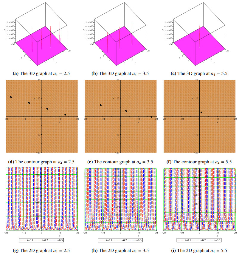
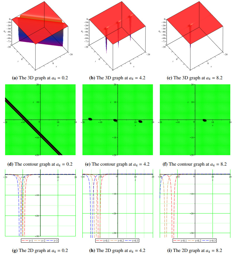
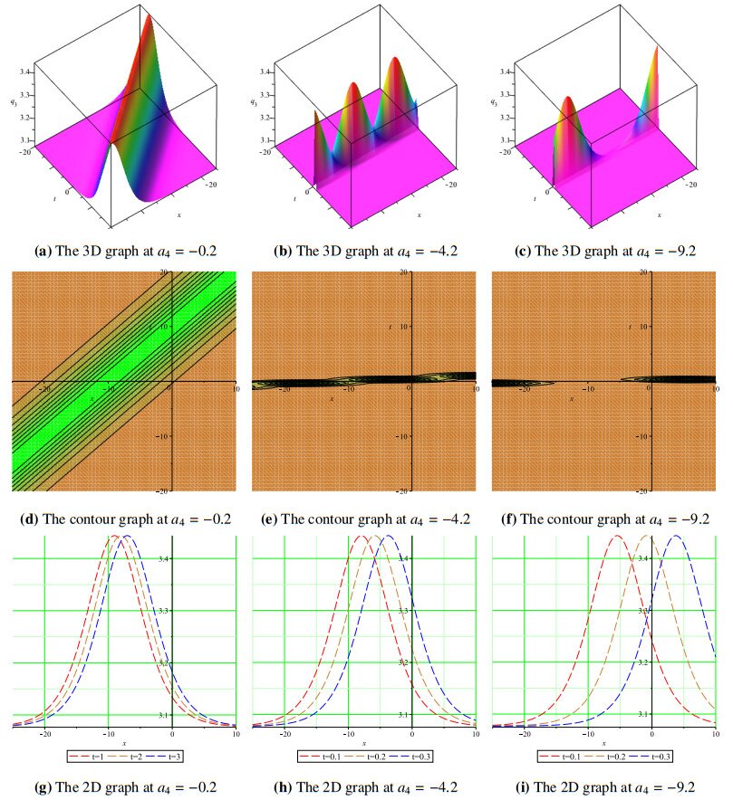
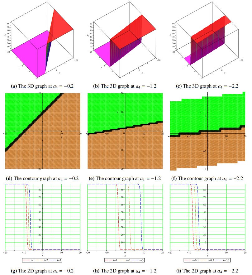
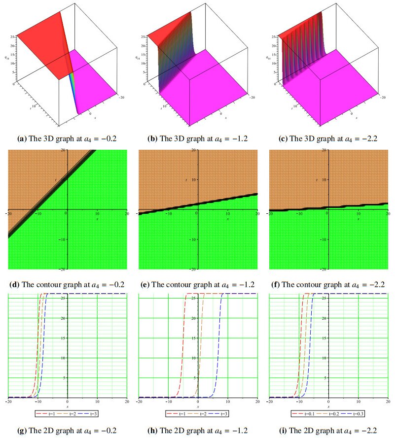
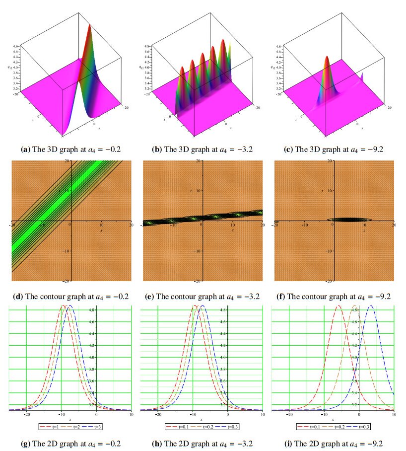
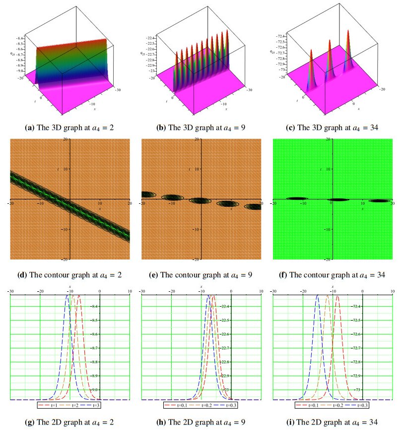
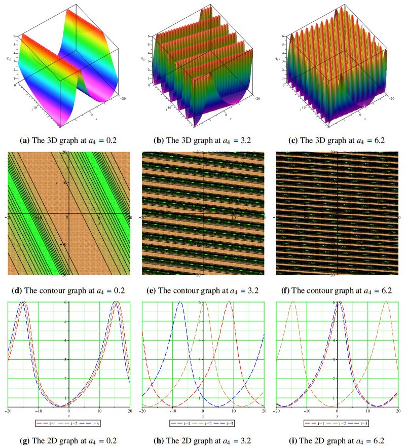
In this paper, diverse wave solutions for the newly introduced (3+1)-dimensional Painlevé-type evolution equation were derived using the improved generalized Riccati equation and generalized Kudryashov methods. This equation is now widely used in soliton theory, nonlinear wave theory, and plasma physics to study instabilities and the evolution of plasma waves. Using these methods, combined with wave transformation and homogeneous balancing techniques, we obtained concise and general wave solutions for the Painlevé-type equation. These solutions included rational exponential, trigonometric, and hyperbolic function solutions. Some of the obtained solutions for the Painlevé-type equation were plotted in terms of 3D, 2D, and contour graphs to depict the various exciting wave patterns that can occur. As the value of the amplitude increased in the investigated solutions, we observed the evolution of dark and bright solutions into rogue waves in the forms of Kuztnetsov-Ma breather and Peregrine-like solitons. Other exciting wave patterns observed in this work included the evolution of kink and multiple wave solitons at different time levels. We believe that the solutions obtained in this paper were concise and more general than existing ones and will be of great use in the study of solitons, nonlinear waves, and plasma physics.
- Painlevé-type equation,
- improved generalized Riccati equation method,
- soliton theory,
- generalized Kudryashov method,
- multiple soliton
Citation: Jamilu Sabi'u, Sekson Sirisubtawee, Surattana Sungnul, Mustafa Inc. Wave dynamics for the new generalized (3+1)-D Painlevé-type nonlinear evolution equation using efficient techniques[J]. AIMS Mathematics, 2024, 9(11): 32366-32398. doi: 10.3934/math.20241552

Related Papers:

Abstract

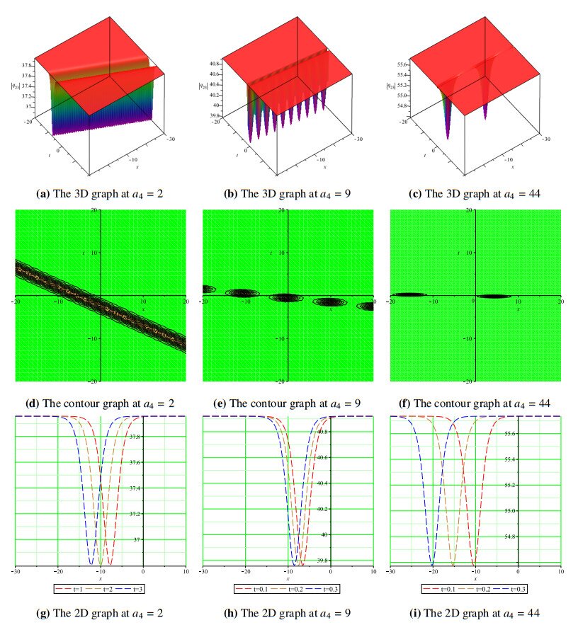
In this paper, diverse wave solutions for the newly introduced (3+1)-dimensional Painlevé-type evolution equation were derived using the improved generalized Riccati equation and generalized Kudryashov methods. This equation is now widely used in soliton theory, nonlinear wave theory, and plasma physics to study instabilities and the evolution of plasma waves. Using these methods, combined with wave transformation and homogeneous balancing techniques, we obtained concise and general wave solutions for the Painlevé-type equation. These solutions included rational exponential, trigonometric, and hyperbolic function solutions. Some of the obtained solutions for the Painlevé-type equation were plotted in terms of 3D, 2D, and contour graphs to depict the various exciting wave patterns that can occur. As the value of the amplitude increased in the investigated solutions, we observed the evolution of dark and bright solutions into rogue waves in the forms of Kuztnetsov-Ma breather and Peregrine-like solitons. Other exciting wave patterns observed in this work included the evolution of kink and multiple wave solitons at different time levels. We believe that the solutions obtained in this paper were concise and more general than existing ones and will be of great use in the study of solitons, nonlinear waves, and plasma physics.

References

[1]	S. Raza, A. Rauf, J. Sabi'u, A. Shah, A numerical method for solution of incompressible Navier-Stokes equations in streamfunction-vorticity formulation, Comput. Math. Methods, 3 (2021), e1188. https://doi.org/10.1002/cmm4.1188 doi: 10.1002/cmm4.1188
[2]	D. J. Zhang, S. L. Zhao, Y. Y. Sun, J. Zhou, Solutions to the modified Korteweg-de Vries equation, Rev. Math. Phys., 26 (2014), 1430006. https://doi.org/10.1142/S0129055X14300064 doi: 10.1142/S0129055X14300064
[3]	V. Novikov, Generalizations of the Camassa-Holm equation, J. Phys. A Math. Theor., 42 (2009), 342002. https://doi.org/10.1088/1751-8113/42/34/342002 doi: 10.1088/1751-8113/42/34/342002
[4]	Z. Y. Yan, Abundant symmetries and exact compacton-like structures in the two-parameter family of the Estevez-Mansfield-Clarkson equations, Commun. Theor. Phys., 37 (2002), 27. https://doi.org/10.1088/0253-6102/37/1/27 doi: 10.1088/0253-6102/37/1/27
[5]	L. V. Bogdanov, V. E. Zakharov, The Boussinesq equation revisited, Phys. D, 165 (2002), 137–162. https://doi.org/10.1016/S0167-2789(02)00380-9 doi: 10.1016/S0167-2789(02)00380-9
[6]	J. Y. Yang, W. X. Ma, Abundant lump-type solutions of the Jimbo-Miwa equation in (3+1)-dimensions, Comput. Math. Appl., 73 (2017), 220–225. https://doi.org/10.1016/j.camwa.2016.11.007 doi: 10.1016/j.camwa.2016.11.007
[7]	M. P. Bonkile, A. Awasthi, C. Lakshmi, V. Mukundan, V. S. Aswin, A systematic literature review of Burgers' equation with recent advances, Pramana, 90 (2018), 1–21. https://doi.org/10.1007/s12043-018-1559-4 doi: 10.1007/s12043-018-1559-4
[8]	G. Biondini, D. Pelinovsky, Kadomtsev-Petviashvili equation, Scholarpedia, 3 (2008), 6539. https://doi.org/10.4249/scholarpedia.6539 doi: 10.4249/scholarpedia.6539
[9]	A. Hasegawa, Soliton-based optical communications: an overview, IEEE J. Sel. Top. Quantum Electron., 6 (2000), 1161–1172. https://doi.org/10.1109/2944.902164 doi: 10.1109/2944.902164
[10]	S. B. Wang, G. L. Ma, X. Zhang, D. Y. Zhu, Dynamic behavior of optical soliton interactions in optical communication systems, Chinese Phys. Lett., 39 (2022), 114202. https://doi.org/10.1088/0256-307X/39/11/114202 doi: 10.1088/0256-307X/39/11/114202
[11]	I. Nikolkina, I. Didenkulova, Rogue waves in 2006–2010, Nat. Hazards Earth Syst. Sci., 11 (2011), 2913–2924. https://doi.org/10.5194/nhess-11-2913-2011
[12]	S. Residori, M. Onorato, U. Bortolozzo, F. T. Arecchi, Rogue waves: a unique approach to multidisciplinary physics, Contemp. Phys., 58 (2017), 53–69. https://doi.org/10.1080/00107514.2016.1243351 doi: 10.1080/00107514.2016.1243351
[13]	X. Wang, L. Wang, C. Liu, B. W. Guo, J. Wei, Rogue waves, semirational rogue waves and W-shaped solitons in the three-level coupled Maxwell-Bloch equations, Commun. Nonlinear Sci. Numer. Simul., 107 (2022), 106172. https://doi.org/10.1016/j.cnsns.2021.106172 doi: 10.1016/j.cnsns.2021.106172
[14]	L. F. Li, Y. Y. Xie, Rogue wave solutions of the generalized (3+1)-dimensional Kadomtsev-Petviashvili equation, Chaos Soliton Fract., 147 (2021), 110935. https://doi.org/10.1016/j.chaos.2021.110935 doi: 10.1016/j.chaos.2021.110935
[15]	B. Mohan, S. Kumar, R. Kumar, Higher-order rogue waves and dispersive solitons of a novel P-type (3+1)-D evolution equation in soliton theory and nonlinear waves, Nonlinear Dyn., 111 (2023), 20275–20288. https://doi.org/10.1007/s11071-023-08938-1 doi: 10.1007/s11071-023-08938-1
[16]	D. Baldwin, W. Hereman, Symbolic software for the Painlevé test of nonlinear ordinary and partial differential equations, J. Nonlinear Math. Phys., 13 (2006), 90–110. https://doi.org/10.2991/jnmp.2006.13.1.8 doi: 10.2991/jnmp.2006.13.1.8
[17]	M. Şenol, M. Ö. Erol, New conformable P-type $(3+1) $-dimensional evolution equation and its analytical and numerical solutions, J. New Theory, 2024, 71–88. https://doi.org/10.53570/jnt.1420224
[18]	S. Kumar, B. Mohan, A novel analysis of Cole-Hopf transformations in different dimensions, solitons, and rogue waves for a (2+1)-dimensional shallow water wave equation of ion-acoustic waves in plasmas, Phys. Fluids, 35 (2023), 127128. https://doi.org/10.1063/5.0185772 doi: 10.1063/5.0185772
[19]	S. K. Dhiman, S. Kumar, Analyzing specific waves and various dynamics of multi-peakons in (3+1)-dimensional p-type equation using a newly created methodology, Nonlinear Dyn., 112 (2024), 10277–10290. https://doi.org/10.1007/s11071-024-09588-7 doi: 10.1007/s11071-024-09588-7
[20]	U. K. Mandal, A. Das, W. X. Ma, Integrability, breather, rogue wave, lump, lump-multi-stripe, and lump-multi-soliton solutions of a (3+1)-dimensional nonlinear evolution equation, Phys. Fluids, 36 (2024), 037151. https://doi.org/10.1063/5.0195378 doi: 10.1063/5.0195378
[21]	S. Kumar, B. Mohan, Bilinearization and new center-controlled N-rogue solutions to a (3+1)-dimensional generalized KdV-type equation in plasmas via direct symbolic approach, Nonlinear Dyn., 112 (2024), 11373–11382. https://doi.org/10.1007/s11071-024-09626-4 doi: 10.1007/s11071-024-09626-4
[22]	M. N. Rafiq, H. B. Chen, Dynamics of three-wave solitons and other localized wave solutions to a new generalized (3+1)-dimensional P-type equation, Chaos Soliton Fract., 180 (2024), 114604. https://doi.org/10.1016/j.chaos.2024.114604 doi: 10.1016/j.chaos.2024.114604
[23]	A. Fahim, N. Touzi, X. Warin, A probabilistic numerical method for fully nonlinear parabolic PDEs, Ann. Appl. Probab., 21 (2011), 1322–1364. https://doi.org/10.1214/10-AAP723 doi: 10.1214/10-AAP723
[24]	J. Y. Wang, J. Cockayne, O. Chkrebtii, T. J. Sullivan, C. J. Oates, Bayesian numerical methods for nonlinear partial differential equations, Statist. Comput., 31 (2021), 1–20. https://doi.org/10.1007/s11222-021-10030-w doi: 10.1007/s11222-021-10030-w
[25]	S. N. Antontsev, J. I. Díaz, S. Shmarev, A. J. Kassab, Energy methods for free boundary problems: applications to nonlinear PDEs and fluid mechanics. Progress in nonlinear differential equations and their applications, Vol 48, Appl. Mech. Rev., 55 (2002), B74–B75. https://doi.org/10.1115/1.1483358 doi: 10.1115/1.1483358
[26]	G. M. Yao, C. S. Chen, H. Zheng, A modified method of approximate particular solutions for solving linear and nonlinear PDEs, Numer. Methods Partial Differ. Equ., 33 (2017), 1839–1858. https://doi.org/10.1002/num.22161 doi: 10.1002/num.22161
[27]	S. Garg, M. Pant, Meshfree methods: a comprehensive review of applications, Int. J. Comput. Methods, 15 (2018), 1830001. https://doi.org/10.1142/S0219876218300015 doi: 10.1142/S0219876218300015
[28]	J. A. Hernández, A. Giuliodori, E. Soudah, Empirical interscale finite element method (EIFEM) for modeling heterogeneous structures via localized hyperreduction, Comput. Methods Appl. Mech. Eng., 418 (2024), 116492. https://doi.org/10.1016/j.cma.2023.116492 doi: 10.1016/j.cma.2023.116492
[29]	H. Khalilzadeh, A. Habibzadeh-Sharif, M. Z. Bideskan, N. Anvarhaghighi, Design of a triple-band black phosphorus-based perfect absorber and full-wave analysis using the semi-analytical method of lines, Photonics Nanostruct., 53 (2023), 101112. https://doi.org/10.1016/j.photonics.2023.101112 doi: 10.1016/j.photonics.2023.101112
[30]	M. T. Hoang, M. Ehrhardt, A second-order nonstandard finite difference method for a general Rosenzweig-MacArthur predator-prey model, J. Comput. Appl. Math., 444 (2024), 115752. https://doi.org/10.1016/j.cam.2024.115752 doi: 10.1016/j.cam.2024.115752
[31]	A. J. M. Jawad, M. D. Petković, A. Biswas, Modified simple equation method for nonlinear evolution equations, Appl. Math. Comput., 217 (2010), 869–877. https://doi.org/10.1016/j.amc.2010.06.030 doi: 10.1016/j.amc.2010.06.030
[32]	W. X. Ma, J. H. Lee, A transformed rational function method and exact solutions to the 3+1 dimensional Jimbo-Miwa equation, Chaos Soliton Fract., 42 (2009), 1356–1363. https://doi.org/10.1016/j.chaos.2009.03.043 doi: 10.1016/j.chaos.2009.03.043
[33]	E. Yusufoğlu, New solitonary solutions for the MBBM equations using Exp-function method, Phys. Lett. A, 372 (2008), 442–446. https://doi.org/10.1016/j.physleta.2007.07.062 doi: 10.1016/j.physleta.2007.07.062
[34]	E. Fan, Extended tanh-function method and its applications to nonlinear equations, Phys. Lett. A, 277 (2000), 212–218. https://doi.org/10.1016/S0375-9601(00)00725-8 doi: 10.1016/S0375-9601(00)00725-8
[35]	Y. T. Gao, B. Tian, Generalized hyperbolic-function method with computerized symbolic computation to construct the solitonic solutions to nonlinear equations of mathematical physics, Comput. Phys. Commun., 133 (2001), 158–164. https://doi.org/10.1016/S0010-4655(00)00168-5 doi: 10.1016/S0010-4655(00)00168-5
[36]	M. Kaplan, A. Bekir, A. Akbulut, A generalized Kudryashov method to some nonlinear evolution equations in mathematical physics, Nonlinear Dyn., 85 (2016), 2843–2850. https://doi.org/10.1007/s11071-016-2867-1 doi: 10.1007/s11071-016-2867-1
[37]	L. Akinyemi, Two improved techniques for the perturbed nonlinear Biswas-Milovic equation and its optical solitons, Optik, 243 (2021), 167477. https://doi.org/10.1016/j.ijleo.2021.167477 doi: 10.1016/j.ijleo.2021.167477
[38]	U. A. Muhammad, J. Sabi'u, S. Salahshour, H. Rezazadeh, Soliton solutions of (2+1) complex modified Korteweg-de Vries system using improved Sardar method, Opt. Quantum Electron., 56 (2024), 802. https://doi.org/10.1007/s11082-024-06591-5 doi: 10.1007/s11082-024-06591-5
[39]	Sirendaoreji, S. Jiong, Auxiliary equation method for solving nonlinear partial differential equations, Phys. Lett. A, 309 (2003), 387–396. https://doi.org/10.1016/S0375-9601(03)00196-8 doi: 10.1016/S0375-9601(03)00196-8
[40]	I. S. Ibrahim, J. Sabi'u, Y. Y. Gambo, S. Rezapour, M. Inc, Dynamic soliton solutions for the modified complex Korteweg-de Vries system, Opt. Quantum Electron., 56 (2024), 954. https://doi.org/10.1007/s11082-024-06821-w doi: 10.1007/s11082-024-06821-w
[41]	M. I. Khan, S. Asghar, J. Sabi'u, Jacobi elliptic function expansion method for the improved modified Kortwedge-de Vries equation, Opt. Quantum Electron., 54 (2022), 734. https://doi.org/10.1007/s11082-022-04109-5 doi: 10.1007/s11082-022-04109-5
[42]	H. Rezazadeh, J. Sabi'u, R. M. Jena, S. Chakraverty, New optical soliton solutions for Triki-Biswas model by new extended direct algebraic method, Modern Phys. Lett. B, 34 (2020), 2150023. https://doi.org/10.1142/S0217984921500238 doi: 10.1142/S0217984921500238
[43]	J. Sabi'u, S. Sirisubtawee, M. Inc, Optical soliton solutions for the Chavy-Waddy-Kolokolnikov model for bacterial colonies using two improved methods, J. Appl. Math. Comput., 2024, 1–24. https://doi.org/10.1007/s12190-024-02169-2
[44]	S. T. Demiray, Y. Pandir, H. Bulut, Generalized Kudryashov method for time-fractional differential equations, Abstr. Appl. Anal., 2014 (2014), 901540. https://doi.org/10.1155/2014/901540
[45]	N. A. Kudryashov, Simplest equation method to look for exact solutions of nonlinear differential equations, Chaos Soliton Fract., 24 (2005), 1217–1231. https://doi.org/10.1016/j.chaos.2004.09.109 doi: 10.1016/j.chaos.2004.09.109
[46]	E. W. Weisstein, CRC concise encyclopedia of mathematics, New York: Chapman and Hall/CRC, 2002. https://doi.org/10.1201/9781420035223

Reader Comments

Your name:*

Email:*
© 2024 the Author(s), licensee AIMS Press. This is an open access article distributed under the terms of the Creative Commons Attribution License (http://creativecommons.org/licenses/by/4.0)