Coronavirus dynamics, infections and preventive interventions using fractional-calculus analysis

Salah Boulaaras; Ziad Ur Rehman; Farah Aini Abdullah; Rashid Jan; Mohamed Abdalla; Asif Jan; Salah Boulaaras; Ziad Ur Rehman; Farah Aini Abdullah; Rashid Jan; Mohamed Abdalla; Asif Jan

doi:10.3934/math.2023436

AIMS Mathematics

2023, Volume 8, Issue 4: 8680-8701. doi: 10.3934/math.2023436

Previous Article Next Article

Research article

Coronavirus dynamics, infections and preventive interventions using fractional-calculus analysis

1.
Department of Mathematics, College of Sciences and Arts, ArRass, Qassim University, Saudi Arabia
2.
Department of Mathematics, University of Swabi, Swabi 23561, Pakistan
3.
School of Mathematical Sciences, Universiti Sains Malaysia, 11800 USM Penang, Malaysia
4.
Mathematics Department, College of Science, King Khalid University, Abha, Saudi Arabia
5.
Department of Pathogenic Microbiology Immunology, School of Basic Medical Sciences, Xiaan Jiaotong University, Xiaan 710061, China

Received: 29 November 2022 Revised: 11 January 2023 Accepted: 17 January 2023 Published: 07 February 2023
MSC : 4C05, 92D25

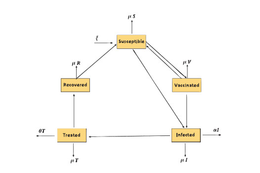
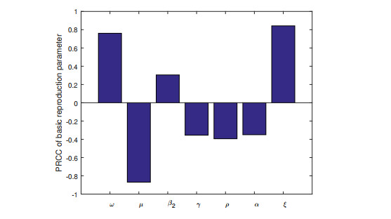
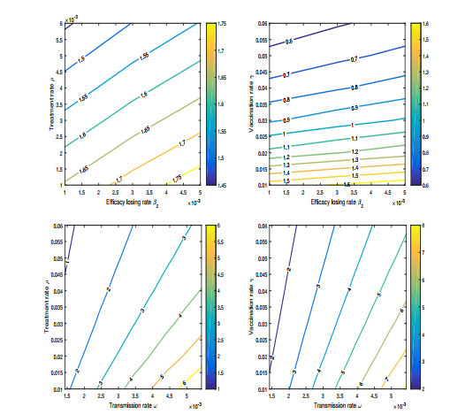
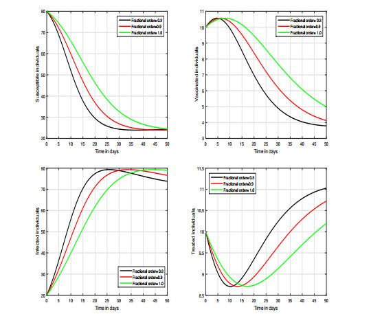
In this research work, we construct an epidemic model to understand COVID-19 transmission vaccination and therapy considerations. The model's equilibria were examined, and the reproduction parameter was calculated via a next-generation matrix method, symbolized by $ \mathcal{R}_0 $. We have shown that the infection-free steady state of our system is locally asymptotically stable for $ \mathcal{R}_0 < 1 $. Also, the local asymptotic stability of the endemic steady state has been established for $ \mathcal{R}_0 > 1 $. We have used a partial rank correlation coefficient method for sensitivity analysis of the threshold parameter $ \mathcal{R}_0 $. The contribution of vaccination to the threshold parameter is explored through graphical results. In addition to this, the uniqueness and existence of the solution to the postulated model of COVID-19 infection is shown. We ran various simulations of the proposed COVID-19 dynamics with varied input parameters to scrutinize the complex dynamics of COVID-19 infection. We illustrated the variation in the dynamical behavior of the system with different values of the input parameters. The key factors of the system are visualized for the public health officials for the control of the infection.
- COVID-19 infection,
- mathematical model,
- vaccination,
- fractional dynamics,
- stability results,
- dynamical behavior
Citation: Salah Boulaaras, Ziad Ur Rehman, Farah Aini Abdullah, Rashid Jan, Mohamed Abdalla, Asif Jan. Coronavirus dynamics, infections and preventive interventions using fractional-calculus analysis[J]. AIMS Mathematics, 2023, 8(4): 8680-8701. doi: 10.3934/math.2023436

Related Papers:

Abstract

In this research work, we construct an epidemic model to understand COVID-19 transmission vaccination and therapy considerations. The model's equilibria were examined, and the reproduction parameter was calculated via a next-generation matrix method, symbolized by $ \mathcal{R}_0 $. We have shown that the infection-free steady state of our system is locally asymptotically stable for $ \mathcal{R}_0 < 1 $. Also, the local asymptotic stability of the endemic steady state has been established for $ \mathcal{R}_0 > 1 $. We have used a partial rank correlation coefficient method for sensitivity analysis of the threshold parameter $ \mathcal{R}_0 $. The contribution of vaccination to the threshold parameter is explored through graphical results. In addition to this, the uniqueness and existence of the solution to the postulated model of COVID-19 infection is shown. We ran various simulations of the proposed COVID-19 dynamics with varied input parameters to scrutinize the complex dynamics of COVID-19 infection. We illustrated the variation in the dynamical behavior of the system with different values of the input parameters. The key factors of the system are visualized for the public health officials for the control of the infection.

References

[1]	V. D. Ashwlayan, C. Antlash, M. Imran, S. M. B. Asdaq, M. K. Alshammari, M. Alomani, et al., Insight into the biological impact of COVID-19 and its vaccines on human health, Saudi J. Biol. Sci., 29 (2022), 3326–3337. https://doi.org/10.1016/j.sjbs.2022.02.010 doi: 10.1016/j.sjbs.2022.02.010
[2]	A. I. Shahin, S. Almotairi, A deep learning BiLSTM encoding-decoding model for COVID-19 pandemic spread forecasting, Fractal Fract., 5 (2021), 175. https://doi.org/10.3390/fractalfract5040175 doi: 10.3390/fractalfract5040175
[3]	J. Wang, J. Pang, X. Liu, Modelling diseases with relapse and nonlinear incidence of infection: a multi-group epidemic model, J. Biol. Dynam., 8 (2014), 99–116. https://doi.org/10.1080/17513758.2014.912682 doi: 10.1080/17513758.2014.912682
[4]	N. Ma, W. Ma, Z. Li, Multi-model selection and analysis for COVID-19, Fractal Fract., 5 (2021), 120. https://doi.org/10.3390/fractalfract5030120 doi: 10.3390/fractalfract5030120
[5]	R. Jan, S. Boulaaras, Analysis of fractional-order dynamics of dengue infection with non-linear incidence functions, T. I. Meas. Control, 44 (2022). https://doi.org/10.1177/01423312221085049
[6]	S. Boulaaras, R. Jan, A. Khan, M. Ahsan, Dynamical analysis of the transmission of dengue fever via Caputo-Fabrizio fractional derivative, Chaos Soliton. Fract., 8 (2022), 100072. https://doi.org/10.1016/j.csfx.2022.100072 doi: 10.1016/j.csfx.2022.100072
[7]	K. Prem, Y. Liu, T. W. Russell, A. J. Kucharski, R. M. Eggo, N. Davies, et al., The effect of control strategies to reduce social mixing on outcomes of the COVID-19 epidemic in Wuhan, China: a modelling study, Lancet Public Health, 5 (2020), e261–e270. https://doi.org/10.1016/S2468-2667(20)30073-6 doi: 10.1016/S2468-2667(20)30073-6
[8]	N. Lurie, M. Saville, R. Hatchett, J. Halton, Developing COVID-19 vaccines at pandemic speed, New Eng. J. Med., 382 (2020), 1969–1973. https://doi.org/10.1056/NEJMp2005630 doi: 10.1056/NEJMp2005630
[9]	F. Amanat, F. Krammer, SARS-CoV-2 vaccines: status report, Immunity, 52 (2020), 583–589. https://doi.org/10.1016/j.immuni.2020.03.007 doi: 10.1016/j.immuni.2020.03.007
[10]	J. E. Aledort, N. Lurie, J. Wasserman, S. A. Bozzette, Non-pharmaceutical public health interventions for pandemic influenza: an evaluation of the evidence base, BMC Public Health, 7 (2007), 1–9. https://doi.org/10.1186/1471-2458-7-208 doi: 10.1186/1471-2458-7-208
[11]	T. M. Chen, J. Rui, Q. P. Wang, Z. Y. Zhao, J. A. Cui, A mathematical model for simulating the phase-based transmissibility of a novel coronavirus, Infect. Dis. Poverty, 9 (2020), 24. https://doi.org/10.1186/s40249-020-00640-3 doi: 10.1186/s40249-020-00640-3
[12]	M. A. Khan, A. Atangana, Modeling the dynamics of novel coronavirus (2019-nCov) with fractional derivative, Alex. Eng. J., 59 (2020), 2379–2389. https://doi.org/10.1016/j.aej.2020.02.033 doi: 10.1016/j.aej.2020.02.033
[13]	J. M. Read, J. R. Bridgen, D. A. Cummings, A. Ho, C. P. Jewell, Novel coronavirus 2019-nCoV: Early estimation of epidemiological parameters and epidemic predictions, Philos. T. R. Soc. B, 376 (2020). https://doi.org/10.1098/rstb.2020.0265
[14]	A. R. Tuite, D. N. Fisman, A. L. Greer, Mathematical modelling of COVID-19 transmission and mitigation strategies in the population of Ontario, CMAJ, 192 (2020), E497–E505. https://doi.org/10.1503/cmaj.200476 doi: 10.1503/cmaj.200476
[15]	O. Pinto Neto, D. M. Kennedy, J. C. Reis, Y. Wang, A. C. B. Brizzi, G. J. Zambrano, et al., Mathematical model of COVID-19 intervention scenarios for Sao PauloBrazil, Nat. Commun., 12 (2021), 418. https://doi.org/10.1038/s41467-020-20687-y doi: 10.1038/s41467-020-20687-y
[16]	O. Nave, U. Shemesh, I. HarTuv, Applying Laplace Adomian decomposition method (LADM) for solving a model of COVID-19, Comput. Method. Biomec., 24 (2021), 1618–1628. https://doi.org/10.1080/10255842.2021.1904399 doi: 10.1080/10255842.2021.1904399
[17]	Z. Shah, R. Jan, P. Kumam, W. Deebani, M. Shutaywi, Fractional dynamics of HIV with source term for the supply of new CD4+ T-cells depending on the viral load via Caputo-Fabrizio derivative, Molecules, 26 (2021), 1806. https://doi.org/10.3390/molecules26061806 doi: 10.3390/molecules26061806
[18]	T. Q. Tang, Z. Shah, R. Jan, E. Alzahrani, Modeling the dynamics of tumorimmune cells interactions via fractional calculus, Eur. Phys. J. Plus, 137 (2022), 367. https://doi.org/10.1140/epjp/s13360-022-02591-0 doi: 10.1140/epjp/s13360-022-02591-0
[19]	S. Qureshi, A. Yusuf, Fractional derivatives applied to MSEIR problems: comparative study with real world data, Eur. Phys. J. Plus, 134 (2019), 171. https://doi.org/10.1140/epjp/i2019-12661-7 doi: 10.1140/epjp/i2019-12661-7
[20]	S. Qureshi, R. Jan, Modeling of measles epidemic with optimized fractional order under Caputo differential operator, Chaos Soliton. Fract., 145 (2021), 110766. https://doi.org/10.1016/j.chaos.2021.110766 doi: 10.1016/j.chaos.2021.110766
[21]	S. Kumar, R. P. Chauhan, S. Momani, S. Hadid, Numerical investigations on COVID-19 model through singular and non-singular fractional operators, Numer. Meth. Part. Differ. Equ., 2020. https://doi.org/10.1002/num.22707
[22]	A. Atangana, S. İĞret araz, A novel COVID-19 model with fractional differential operators with singular and non-singular kernels: analysis and numerical scheme based on Newton polynomial, Alex. Eng. J., 60 (2021), 3781–3806. https://doi.org/10.1016/j.aej.2021.02.016 doi: 10.1016/j.aej.2021.02.016
[23]	R. Jan, A. Khurshaid, H. Alotaibi, M. Inc, A robust study of the transmission dynamics of syphilis infection through non-integer derivative, AIMS Math., 8 (2023), 6206–6232. https://doi.org/10.3934/math.2023314 doi: 10.3934/math.2023314
[24]	O. A. Omar, R. A. Elbarkouky, H. M. Ahmed, Fractional stochastic modelling of COVID-19 under wide spread of vaccinations: Egyptian case study, Alex. Eng. J., 61 (2022), 8595–8609. https://doi.org/10.1016/j.aej.2022.02.002 doi: 10.1016/j.aej.2022.02.002
[25]	O. A. Omar, Y. Alnafisah, R. A. Elbarkouky, H. M. Ahmed, COVID-19 deterministic and stochastic modelling with optimized daily vaccinations in Saudi Arabia, Results Phys., 28 (2021), 104629. https://doi.org/10.1016/j.rinp.2021.104629 doi: 10.1016/j.rinp.2021.104629
[26]	M. Caputo, M. Fabrizio, A new definition of fractional derivative without singular kernel, Progr. Fract. Differ. Appl., 1 (2015), 73–85. http://dx.doi.org/10.12785/pfda/010201 doi: 10.12785/pfda/010201
[27]	J. Losada, J. J. Nieto, Properties of a new fractional derivative without singular kernel, Progr. Fract. Differ. Appl., 1 (2015), 87–92. http://dx.doi.org/10.12785/pfda/010202 doi: 10.12785/pfda/010202
[28]	R. Jan, M. A. Khan, Y. Khan, S. Ullah, A new model of dengue fever in terms of fractional derivative, Math. Biosci. Eng., 17 (2020), 5267–5288.
[29]	P. Van den Driessche, J. Watmough, Reproduction numbers and sub-threshold endemic equilibria for compartmental models of disease transmission, Math. Biosci., 180 (2002), 29–48. https://doi.org/10.1016/S0025-5564(02)00108-6 doi: 10.1016/S0025-5564(02)00108-6
[30]	C. Castillo-Chavez, Z. Feng, W. Huang, On the computation of R0 and its role on global stability, Mathematical approaches for emerging and re-emerging infection diseases: an introduction, 125 (2002), 31–65.

Reader Comments

Your name:*

Email:*
© 2023 the Author(s), licensee AIMS Press. This is an open access article distributed under the terms of the Creative Commons Attribution License (http://creativecommons.org/licenses/by/4.0)