This paper proposes a modified D-iteration to approximate the solutions of three quasi-nonexpansive multivalued mappings in a real Hilbert space. Due to the incorporation of an inertial step in the iteration, the sequence generated by the modified method converges faster to the common fixed point of the mappings. Furthermore, the generated sequence strongly converges to the required solution using a shrinking technique. Numerical results obtained indicate that the proposed iteration is computationally efficient and outperforms the standard forward-backward with inertial step.
Citation: Anantachai Padcharoen, Kritsana Sokhuma, Jamilu Abubakar. Projection methods for quasi-nonexpansive multivalued mappings in Hilbert spaces[J]. AIMS Mathematics, 2023, 8(3): 7242-7257. doi: 10.3934/math.2023364
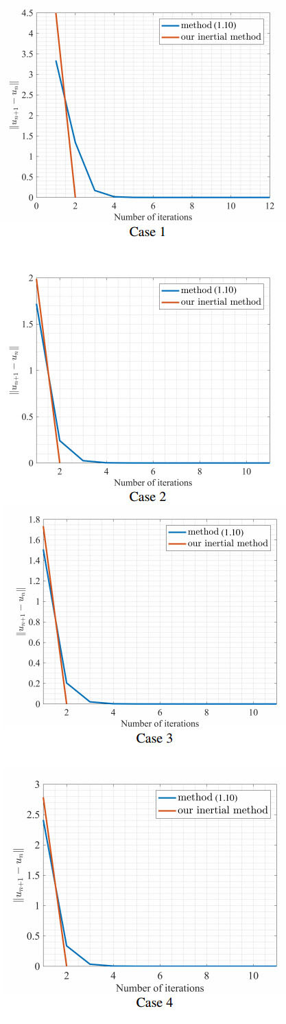
This paper proposes a modified D-iteration to approximate the solutions of three quasi-nonexpansive multivalued mappings in a real Hilbert space. Due to the incorporation of an inertial step in the iteration, the sequence generated by the modified method converges faster to the common fixed point of the mappings. Furthermore, the generated sequence strongly converges to the required solution using a shrinking technique. Numerical results obtained indicate that the proposed iteration is computationally efficient and outperforms the standard forward-backward with inertial step.

| [1] |
F. E. Browder, Nonexpansive nonlinear operators in a Banach space, Proc. Nat. Acad. Sci. USA., 54 (1965), 1041–1044. https://doi.org/10.1073/pnas.54.4.1041 doi: 10.1073/pnas.54.4.1041

|
| [2] |
D. Göhde, Zum prinzip der kontraktiven abbildung, Math. Nachr., 30 (1965), 251–258. https://doi.org/10.1002/mana.19650300312 doi: 10.1002/mana.19650300312
|
| [3] |
S. Reich, Approximate selections, best approximations, fixed points, and invariant sets, J. Math. Anal. Appl., 62 (1978), 104–113. https://doi.org/10.1016/0022-247X(78)90222-6 doi: 10.1016/0022-247X(78)90222-6
|
| [4] | K. Goebel, W. A. Kirk, Topics in metric fixed point theory, Cambridge Studies in Advanced Mathematics, 28, Cambridge: Cambridge University Press, 1990. |
| [5] |
W. A. Kirk, A fixed point theorem for mappings which do not increase distances, Am. Math. Mon., 72 (1965), 1004–1006. https://doi.org/10.2307/2313345 doi: 10.2307/2313345
|
| [6] |
W. R. Mann, Mean value methods in iteration, Proc. Am. Math. Soc., 4 (1953), 506–510. https://doi.org/10.2307/2032162 doi: 10.2307/2032162
|
| [7] |
S. Ishikawa, Fixed points by a new iteration method, Proc. Am. Math. Soc., 44 (1974), 147–150. https://doi.org/10.2307/2039245 doi: 10.2307/2039245
|
| [8] |
M. A. Noor, New approximation schemes for general variational inequalities, J. Math. Anal. Appl., 251 (2000), 217–229. https://doi.org/10.1006/jmaa.2000.7042 doi: 10.1006/jmaa.2000.7042
|
| [9] |
I. Yildirim, M. Özdemir, A new iterative process for common fixed points of finite families of non-self-asymptotically non-expansive mappings, Nonlinear Anal.-Theor., 71 (2009), 991–999. https://doi.org/10.1016/j.na.2008.11.017 doi: 10.1016/j.na.2008.11.017
|
| [10] | P. Sainuan, Rate of convergence of P-iteration and S-iteration for continuous functions on closed intervals, Thai J. Math., 13 (2015), 449–457. |
| [11] |
J. Daengsaen, A. Khemphet, On the rate of convergence of P-iteration, SP-iteration, and D-iteration methods for continuous nondecreasing functions on closed intervals, Abstr. Appl. Anal., 2018 (2018), 7345401. https://doi.org/10.1155/2018/7345401 doi: 10.1155/2018/7345401
|
| [12] | B. T. Polyak, Introduction to optimization, New York: Optimization Software, 1987. |
| [13] |
B. T. Polyak, Some methods of speeding up the convergence of iterative methods, Zh. Vychisl. Mat. Mat. Fiz. 4 (1964), 1–17. https://doi.org/10.1016/0041-5553(64)90137-5 doi: 10.1016/0041-5553(64)90137-5
|
| [14] |
W. Chaolamjiak, D. Yambangwai, H. A. Hammad, Modified hybrid projection methods with SP iterations for quasi-nonexpansive multivalued mappings in Hilbert spaces, B. Iran. Math. Soc., 47 (2021), 1399–1422. https://doi.org/10.1007/s41980-020-00448-9 doi: 10.1007/s41980-020-00448-9
|
| [15] |
P. Cholamjiak, W. Cholamjiak, Fixed point theorems for hybrid multivalued mappings in Hilbert spaces, J. Fixed Point Theory Appl., 18 (2016), 673–688. https://doi.org/10.1007/s11784-016-0302-3 doi: 10.1007/s11784-016-0302-3
|
| [16] | S. Suantai, Weak and strong convergence criteria of Noor iterations for asymptotically nonexpansive mappings, J. Math. Anal. Appl., 311 (2005), 506–517. |
| [17] |
C. Martinez-Yanes, H. K. Xu, Strong convergence of the CQ method for fixed point iteration processes, Nonlinear Anal., 64 (2006), 2400–2411. https://doi.org/10.1016/j.na.2005.08.018 doi: 10.1016/j.na.2005.08.018
|
| [18] |
K. Nakajo, W. Takahashi, Strong convergence theorems for nonexpansive mappings and nonexpansive semigroups, J. Math. Anal. Appl., 279 (2003), 372–379. https://doi.org/10.1016/S0022-247X(02)00458-4 doi: 10.1016/S0022-247X(02)00458-4
|
| [19] |
F. Alvarez, H. Attouch, An inertial proximal method for maximal monotone operators via discretization of a nonlinear oscillator with damping, Set-Valued Anal., 9 (2001), 3–11. https://doi.org/10.1023/A:1011253113155 doi: 10.1023/A:1011253113155
|
| [20] | K. Goebel, S. Reich, Uniform convexity, hyperbolic geometry, and nonexpansive mappings, Monographs and Textbooks in Pure and Applied Mathematics, 83, New York: Marcel Dekker Inc, 1984. https://doi.org/10.1112/blms/17.3.293 |
| [21] | W. Takahashi, Fixed point theorems for new nonlinear mappings in a Hilbert space, J. Nonlinear Convex Anal., 11 (2010), 79–88. |
| [22] |
M. Stošsić, J. Xavier, M. Dodig, Projection on the intersection of convex sets, Linear Algebra Appl., 9 (2016), 191–205. https://doi.org/10.1016/j.laa.2016.07.023 doi: 10.1016/j.laa.2016.07.023
|
Figures(1) / Tables(1)

Anantachai Padcharoen, Kritsana Sokhuma, Jamilu Abubakar. Projection methods for quasi-nonexpansive multivalued mappings in Hilbert spaces[J]. AIMS Mathematics, 2023, 8(3): 7242-7257. doi: 10.3934/math.2023364


 DownLoad: