A solving method for two-dimensional homogeneous system of fuzzy fractional differential equations

Muhammad Akram; Ghulam Muhammad; Tofigh Allahviranloo; Ghada Ali; Muhammad Akram; Ghulam Muhammad; Tofigh Allahviranloo; Ghada Ali

doi:10.3934/math.2023011

AIMS Mathematics

2023, Volume 8, Issue 1: 228-263. doi: 10.3934/math.2023011

Previous Article Next Article

Research article

A solving method for two-dimensional homogeneous system of fuzzy fractional differential equations

1.
Department of Mathematics, University of the Punjab, New Campus, Lahore-54590, Pakistan
2.
Department of Mathematics, Lahore Garrison University, Lahore 54000, Pakistan
3.
Faculty of Engineering and Natural Sciences, Istinye University, Istanbul, Turkey
4.
Department of Mathematics, King Abdulaziz University Jeddah, Saudi Arabia

Received: 23 August 2022 Revised: 20 September 2022 Accepted: 22 September 2022 Published: 28 September 2022
MSC : 34A08, 03E72, 33E12

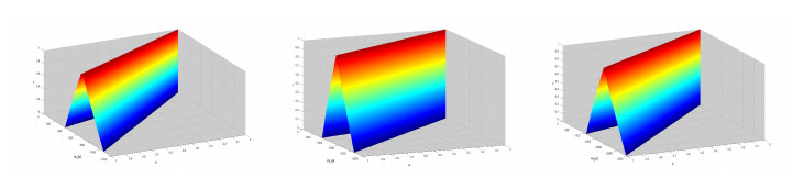
The purpose of this study is to extend and determine the analytical solution of a two-dimensional homogeneous system of fuzzy linear fractional differential equations with the Caputo derivative of two independent fractional orders. We extract two possible solutions to the coupled system under the definition of strongly generalized $ H $-differentiability, uncertain initial conditions and fuzzy constraint coefficients. These potential solutions are determined using the fuzzy Laplace transform. Furthermore, we extend the concept of fuzzy fractional calculus in terms of the Mittag-Leffler function involving triple series. In addition, several important concepts, facts, and relationships are derived and proved as property of boundedness. Finally, to grasp the considered approach, we solve a mathematical model of the diffusion process using proposed techniques to visualize and support theoretical results.
- system of fractional differential equations,
- Mittag-Leffler function,
- fuzzy fractional calculus,
- Caputo fractional derivative,
- diffusion process
Citation: Muhammad Akram, Ghulam Muhammad, Tofigh Allahviranloo, Ghada Ali. A solving method for two-dimensional homogeneous system of fuzzy fractional differential equations[J]. AIMS Mathematics, 2023, 8(1): 228-263. doi: 10.3934/math.2023011

Related Papers:

Abstract

The purpose of this study is to extend and determine the analytical solution of a two-dimensional homogeneous system of fuzzy linear fractional differential equations with the Caputo derivative of two independent fractional orders. We extract two possible solutions to the coupled system under the definition of strongly generalized $ H $-differentiability, uncertain initial conditions and fuzzy constraint coefficients. These potential solutions are determined using the fuzzy Laplace transform. Furthermore, we extend the concept of fuzzy fractional calculus in terms of the Mittag-Leffler function involving triple series. In addition, several important concepts, facts, and relationships are derived and proved as property of boundedness. Finally, to grasp the considered approach, we solve a mathematical model of the diffusion process using proposed techniques to visualize and support theoretical results.

References

[1]	I. Podlubny, Fractional differential equations, Mathematics in Science and Engineering Academic Press, New York, 1999.
[2]	J. Podlubny, Geometric and physical interpretation of fractional integration and fractional differentiation, Fract. Calc. Appl. Anal., 5 (2002), 367–386.
[3]	P. Georgescu, Y. H. Hsieh, Global stability for a virus dynamics model with nonlinear incidence of infection and removal, SIAM J. Appl. Math., 67 (2007), 337–353. https://doi.org/10.1137/060654876 doi: 10.1137/060654876
[4]	I. Muslih, D. Baleanu, E. Rabei, Hamiltonian formulation of classical fields within Riemann-Liouville fractional derivatives, Phys. Scripta, 73 (2006).
[5]	V. Lakshmikantham, S. Leela, J. Vasundhara, Theory of fractional dynamic systems, Cambridge Academic Publishers, Cambridge, UK, 2009.
[6]	M. Dalir, M. Bashour, Applications of fractional calculus, Appl. Math. Sci., 4 (2010).
[7]	D. Baleanu, K. Diethelm, E. Scalas, J. J. Trujillo, Fractional calculus: Models and numerical methods, New York: World Scientific, 2017.
[8]	R. Herrmann, Fractional calculus: An introduction for physicists, 2 Eds., Singapore: World Scientific, 2014.
[9]	R. Hilfer, Applications of fractional calculus in physics, Singapore: World Scientific, 2000.
[10]	H. G. Sun, Y. Zhang, D. Baleanu, W. Chen, Y. Q. Chen, A new collection of real world applications of fractional calculus in science and engineering, Commun. Nonlinear Sci., 64 (2018), 213–231. https://doi.org/10.1016/j.cnsns.2018.04.019 doi: 10.1016/j.cnsns.2018.04.019
[11]	A. A. Kilbas, H. M. Srivastava, J. J. Trujillo, Theory and applications of fractional differential equations, Amsterdam: Elsevier, 2006.
[12]	K. S. Miller, B. Ross, An introduction to the fractional calculus and fractional differential equations, New York: Wiley, 1993.
[13]	I. Podlubny, Fractional differential equations, Academic Press, San Diego, 1999.
[14]	A. Hajipour, H. Tavakoli, Analysis and circuit simulation of a novel nonlinear fractional incommensurate order financial system, Optik, 127 (2016), 10643–10652. https://doi.org/10.1016/j.ijleo.2016.08.098 doi: 10.1016/j.ijleo.2016.08.098
[15]	I. Pan, S. Das, S. Das, Multi-objective active control policy design for commensurate and incommensurate fractional order chaotic financial systems, Appl. Math. Model., 39 (2015), 500–514. https://doi.org/10.1016/j.apm.2014.06.005 doi: 10.1016/j.apm.2014.06.005
[16]	K. Zourmba, A. A. Oumate, B. Gambo, J. Y. Effa, A. Mohamadou, Chaos in the incommensurate fractional order system and circuit simulations, Int. J. Dyn. Control, 7 (2019), 94–111. https://doi.org/10.1007/s40435-018-0442-y doi: 10.1007/s40435-018-0442-y
[17]	X. Wang, Z. Wang, J. Xia, Stability and bifurcation control of a delayed fractional-order eco-epidemiological model with incommensurate orders, J. Franklin I., 356 (2019), 8278–8295. https://doi.org/10.1016/j.jfranklin.2019.07.028 doi: 10.1016/j.jfranklin.2019.07.028
[18]	B. DaȘbaȘi, Stability analysis of the HIV model through incommensurate fractional-order nonlinear system, Chaos Soliton. Fract., 137 (2020), 109870. https://doi.org/10.1016/j.chaos.2020.109870 doi: 10.1016/j.chaos.2020.109870
[19]	S. B. Hadid, Y. F. Luchko, An operational method for solving fractional differential equations of an arbitrary real order, Panam. Math. J., 6 (1996), 207–233.
[20]	R. Hilfer, Y. Luchko, Z. Tomovski, Operational method for the solution of fractional differential equations with generalized Riemann-Liouville fractional derivatives, Fract. Calc. Appl. Anal., 12 (2009), 299–318.
[21]	Y. F. Luchko, R. Gorenflo, An operational method for solving fractional differential equations with Caputo derivatives, Acta Math. Vietnam., 24 (1999), 207–233.
[22]	Y. Luchko, S. Yakubovich, An operational method for solving some classes of integro-differential equations, Differ. Eq., 30 (1994), 269–280.
[23]	A. Omame, D. Okuonghae, U. K. Nwajeri, C. P. Onyenegecha, A fractional-order multi-vaccination model for COVID-19 with non-singular kernel, Alex. Eng. J., 61 (2022), 6089–6104. https://doi.org/10.1016/j.aej.2021.11.037 doi: 10.1016/j.aej.2021.11.037
[24]	J. Singh, Analysis of fractional blood alcohol model with composite fractional derivative, Chaos Soliton. Fract., 140 (2020), 110127. https://doi.org/10.1016/j.chaos.2020.110127 doi: 10.1016/j.chaos.2020.110127
[25]	M. Bhakta, S. Chakraborty, P. Pucci, Fractional Hardy-Sobolev equations with nonhomogeneous terms, Adv. Nonlinear Anal., 10 (2021), 1086–1116. https://doi.org/10.1515/anona-2020-0171 doi: 10.1515/anona-2020-0171
[26]	A. Mohammed, V. D. Radulescu, A. Vitolo, Blow-up solutions for fully nonlinear equations: existence, asymptotic estimates and uniqueness, Adv. Nonlinear Anal., 9 (2020), 39–64. https://doi.org/10.1515/anona-2018-0134 doi: 10.1515/anona-2018-0134
[27]	X. Mingqi, V. D. Radulescu, B. Zhang, Nonlocal Kirchhoff problems with singular exponential nonlinearity, Appl. Math. Optim., 84 (2021), 915–954. https://doi.org/10.1007/s00245-020-09666-3 doi: 10.1007/s00245-020-09666-3
[28]	X. Mingqi, V. D. Radulescu, B. Zhang, Combined effects for fractional Schrödinger-Kirchhoff systems with critical nonlinearities, ESAIM Contr. Optim. Ca., 24 (2018), 1249–1273. https://doi.org/10.1051/cocv/2017036 doi: 10.1051/cocv/2017036
[29]	J. F. Bonder, Z. Cheng, H. Mikayelyan, Optimal rearrangement problem and normalized obstacle problem in the fractional setting, Adv. Nonlinear Anal., 9 (2020), 1592–1606. https://doi.org/10.1515/anona-2020-0067 doi: 10.1515/anona-2020-0067
[30]	A. Fernandez, D. Baleanu, A. S. Fokas, Solving PDEs of fractional order using the unified transform method, Appl. Math. Comput., 339 (2018), 73849. https://doi.org/10.1016/j.amc.2018.07.061 doi: 10.1016/j.amc.2018.07.061
[31]	L. A. Zadeh, Fuzzy sets, Inform. Contr., 8 (1965), 338–353.
[32]	T. Abdeljawad, Fractional difference operators with discrete generalized Mittag-Leffler kernels, Chaos Soliton. Fract., 126 (2019), 315–324. https://doi.org/10.1016/j.chaos.2019.06.012 doi: 10.1016/j.chaos.2019.06.012
[33]	T. Allahviranloo, Fuzzy fractional differential operators and equations, Stud. Fuzz. Soft Comput., 2020,397. https://doi.org/10.1007/978-3-030-51272-9
[34]	O. A. Arqub, Numerical solutions of systems of first-order, two-point BVPs based on the reproducing kernel algorithm, Calcolo, 55 (2018), 1–28. https://doi.org/10.1007/s10092-018-0274-3 doi: 10.1007/s10092-018-0274-3
[35]	O. A. Arqub, B. Maayah, Fitted fractional reproducing kernel algorithm for the numerical solutions of ABC-Fractional Volterra integro-differential equations, Chaos Soliton. Fract., 126 (2019), 394–402. https://doi.org/10.1016/j.chaos.2019.07.023 doi: 10.1016/j.chaos.2019.07.023
[36]	O. A. Arqub, B. Maayah, Numerical solutions of integrodifferential equations of Fredholm operator type in the sense of the Atangana-Baleanu fractional operator, Chaos Soliton. Fract., 117 (2018), 117–124. https://doi.org/10.1016/j.chaos.2018.10.007 doi: 10.1016/j.chaos.2018.10.007
[37]	O. A. Arqub, M. A. Smadi, An adaptive numerical approach for the solutions of fractional advection-diffusion and dispersion equations in singular case under Riesz's derivative operator, Physica A, 540 (2020), 123257. https://doi.org/10.1016/j.physa.2019.123257 doi: 10.1016/j.physa.2019.123257
[38]	M. A. Smadi, O. A. Arqub, Computational algorithm for solving fredholm time-fractional partial integrodifferential equations of dirichlet functions type with error estimates, Appl. Math. Comput., 342 (2019), 280–294. https://doi.org/10.1016/j.amc.2018.09.020 doi: 10.1016/j.amc.2018.09.020
[39]	M. A. Smadi, O. A. Arqub, S. Hadid, An attractive analytical technique for coupled system of fractional partial differential equations in shallow water waves with conformable derivative, Commun. Theor. Phys., 72 (2020), 085001.
[40]	S. Abbasbandy, T. A. Viranloo, Numerical solution of fuzzy differential equation, Math. comput. Appl., 7 (2002), 41–52. https://doi.org/10.3390/mca7010041 doi: 10.3390/mca7010041
[41]	S. S. L. Chang, L. A. Zadeh, On fuzzy mapping and control, IEEE T. Syst. Sci. Cy., 2 (1972), 30–34. https://doi.org/10.1142/9789814261302_0012 doi: 10.1142/9789814261302_0012
[42]	D. Dubios, H. Prade, Towards fuzzy differential calculus part 3: Differentiation, Fuzzy Set. Syst., 8 (1982), 225–233.
[43]	O. Kaleva, Fuzzy differential equations, Fuzzy Set. Syst., 24 (1987), 301–317. https://doi.org/10.1016/0165-0114(87)90029-7 doi: 10.1016/0165-0114(87)90029-7
[44]	O. Kaleva, The Cauchy problem for fuzzy differential equations, Fuzzy Set. Syst., 35 (1990), 389–396. https://doi.org/10.1016/0165-0114(90)90010-4 doi: 10.1016/0165-0114(90)90010-4
[45]	S. Seikkala, On the fuzzy initial value problem, Fuzzy Set. Syst., 24 (1987), 319–330. https://doi.org/10.1016/0165-0114(87)90030-3 doi: 10.1016/0165-0114(87)90030-3
[46]	N. Van Hoa, V. Lupulescu, D. O'Regan, Solving interval-valued fractional initial value problems under Caputo $gH$-fractional differentiability, Fuzzy Set. Syst., 309 (2017), 1–34. https://doi.org/10.1016/j.fss.2016.09.015 doi: 10.1016/j.fss.2016.09.015
[47]	M. Akram, T. Ihsan, T. Allahviranloo, Solving Pythagorean fuzzy fractional differential equations using Laplace transform, Granular Comput., 2022, 1–25. https://doi.org/10.1007/s41066-022-00344-z doi: 10.1007/s41066-022-00344-z
[48]	M. Akram, T. Ihsan, T. Allahviranloo, M. M. A. Al-Shamiri, Analysis on determining the solution of fourth-order fuzzy initial value problem with Laplace operator, Math. Biosci. Eng., 19 (2022), 11868–11902. https://doi.org/10.3934/mbe.2022554 doi: 10.3934/mbe.2022554
[49]	M. Akram, G. Muhammad, T. Allahviranloo, G. Ali, New analysis of fuzzy fractional Langevin differential equations in Caputo's derivative sense, AIMS Math., 7 (2022), 18467–18496. https://doi.org/10.3934/math.20221016 doi: 10.3934/math.20221016
[50]	R. Goetschel Jr, W. Voxman, Elementary fuzzy calculus, Fuzzy set. syst., 18 (1986), 31–43. https://doi.org/10.1016/0165-0114(86)90026-6 doi: 10.1016/0165-0114(86)90026-6
[51]	B. Bede, S. G. Gal, Generalizations of the differentiability of fuzzy-number-valued functions with applications to fuzzy differential equations, Fuzzy Set. Syst., 151 (2005), 581–599. https://doi.org/10.1016/j.fss.2004.08.001 doi: 10.1016/j.fss.2004.08.001
[52]	K. Diethelm, The analysis of fractional differential equations: An application-oriented exposition using differential operators of Caputo type, Springer Science Business Media, 2010. https://doi.org/10.1007/978-3-642-14574-2
[53]	I. Podlubny, Fractional differential equations: An introduction to fractional derivatives, fractional differential equations, to methods of their solution and some of their applications, Elsevier, 1998.
[54]	S. G. Samko, A. A. Kilbas, O. I. Marichev, Fractional integrals and derivatives: Theory and applications, Yverdon: Gordon Breach Science Publishers, 1993.
[55]	S. Salahshour, T. Allahviranloo, S. Abbasbandy, Solving fuzzy fractional differential equations by fuzzy Laplace transforms, Commun. Nonlinear Sci. Numer. Simu., 17 (2012), 1372–1381. https://doi.org/10.1016/j.cnsns.2011.07.005 doi: 10.1016/j.cnsns.2011.07.005
[56]	T. Allahviranloo, M. B. Ahmadi, Fuzzy Laplace transforms, Soft Comput., 14 (2010), 235. https://doi.org/10.1007/s00500-008-0397-6 doi: 10.1007/s00500-008-0397-6
[57]	G. M. Mittag-Leffler, Sur la nouvelle fonction Eα (x). CR Acad. Sci. Paris, 137 (1903), 554–558.
[58]	A. Fernandez, C. K$\ddot{i}$rt, M. A. Özarslan, A naturally emerging bivariate Mittag-Leffler function and associated fractional-calculus operators, Comput. Appl. Math., 39 (2020). https://doi.org/10.1007/s40314-020-01224-5 doi: 10.1007/s40314-020-01224-5
[59]	R. Gorenflo, A. A. Kilbas, F. Mainardi, S. V. Rogosin, Mittag-Leffler functions, related topics and applications, Berlin: Springer-Verlag, 2014. https://doi.org/10.1007/978-3-662-61550-8
[60]	I. T. Huseynov, A. Ahmadova, G. O. Ojo, N. I. Mahmudov, A natural extension of Mittag-Leffler function associated with a triple infinite series. https://doi.org/10.48550/arXiv.2011.03999
[61]	A. Omame, U. K. Nwajeri, M. Abbas, C. P. Onyenegecha, A fractional order control model for Diabetes and COVID-19 co-dynamics with Mittag-Leffler function, Alex. Eng. J., 2022. https://doi.org/10.1016/j.aej.2022.01.012
[62]	R. K. Saxena, S. L. Kalla, R. Saxena, Multivariate analogue of generalised Mittag-Leffler function, Integr. Transf. Spec. F., 22 (2011), 533–548. https://doi.org/10.1080/10652469.2010.533474 doi: 10.1080/10652469.2010.533474
[63]	A. Ahmadova, I. T. Huseynov, A. Fernandez, N. I. Mahmudov, Trivariate Mittag-Leffler functions used to solve multi-order systems of fractional differential equations, Commun. Nonlinear Sci. Numer. Simu., 97 (2021), 105735. https://doi.org/10.1016/j.cnsns.2021.105735 doi: 10.1016/j.cnsns.2021.105735
[64]	O. A. Arqub, Numerical solutions for the Robin time-fractional partial differential equations of heat and fluid flows based on the reproducing kernel algorithm, Int. J. Numer. Method. H., 28 (2018), 828–856. https://doi.org/10.1108/HFF-07-2016-0278 doi: 10.1108/HFF-07-2016-0278
[65]	D. Takaci, A. Takaci, A. Takaci, On the operational solutions of fuzzy fractional differential equations, Fract. Calc. Appl. Anal., 17 (2014), 1100–1113. https://doi.org/10.2478/s13540-014-0216-y doi: 10.2478/s13540-014-0216-y
[66]	B. Kolman, D. Hill, Elementary linear algebra with applications, 9 Eds., Pearson, 2007.
[67]	E. Hernández-Balaguera, E. López-Dolado, J. L. Polo, In vivo rat spinal cord and striated muscle monitoring using the current interruption method and bioimpedance measurements, J. Electrochem. Soc., 165 (2018), G3099.
[68]	R. L. Magin, Fractional calculus models of complex dynamics in biological tissues, Comput. Math. Appl., 59 (2010), 1586–1593. https://doi.org/10.1016/j.camwa.2009.08.039 doi: 10.1016/j.camwa.2009.08.039
[69]	E. Hernández-Balaguera, Numerical approximations on the transient analysis of bioelectric phenomena at long time scales via the Mittag-Leffler function, Chaos Soliton. Fract., 145 (2021), 110768. https://doi.org/10.1016/j.chaos.2021.110768 doi: 10.1016/j.chaos.2021.110768
[70]	T. R. Prabhakar, A singular integral equation with a generalized Mittag-Leffler function in the kernel, Yokohama Math. J., 19 (1971), 715.

Reader Comments

Your name:*

Email:*
© 2023 the Author(s), licensee AIMS Press. This is an open access article distributed under the terms of the Creative Commons Attribution License (http://creativecommons.org/licenses/by/4.0)