Dynamics of fractional order delay model of coronavirus disease

Lei Zhang; Mati Ur Rahman; Shabir Ahmad; Muhammad Bilal Riaz; Fahd Jarad; Lei Zhang; Mati Ur Rahman; Shabir Ahmad; Muhammad Bilal Riaz; Fahd Jarad

doi:10.3934/math.2022234

AIMS Mathematics

2022, Volume 7, Issue 3: 4211-4232. doi: 10.3934/math.2022234

Previous Article Next Article

Research article Special Issues

Dynamics of fractional order delay model of coronavirus disease

1.
Department of Mathematics, Hanshan Normal University, Chaozhou, 521041, China
2.
Department of Mathematics, Shanghai Jiao Tong University, 800 Dongchuan Road Shanghai, China
3.
Department of Mathematics, University of Malakand, Chakdara Dir (L), Khyber Pakhtunkhwa, Pakistan
4.
Department of Automation, Biomechanics and Mechatronics, Lodz University of Technology, 1/15 Stefanowskiego St., 90924, Lodz, Poland
5.
Department of Mathematics, University of Management and Technology, Lahore 54770, Pakistan
6.
Department of Mathematics, Cankaya University, Etimesgut 06790, Ankara, Turkey
7.
King Abdulaziz University Jeddah, Saudia Arabia
8.
Department of Medical Research, China Medical University, Taichung 40402, Taiwan

Received: 19 September 2021 Revised: 05 December 2021 Accepted: 09 December 2021 Published: 17 December 2021
MSC : 92B05, 92C10, 92C15

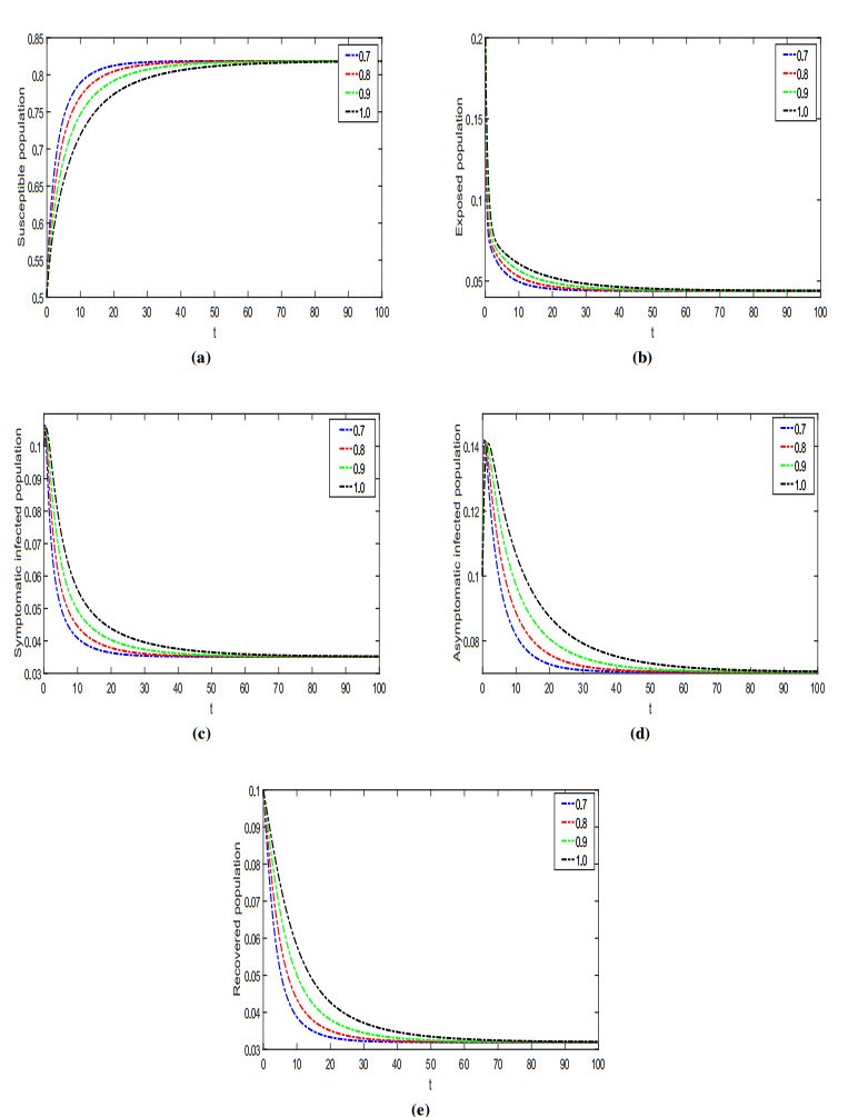
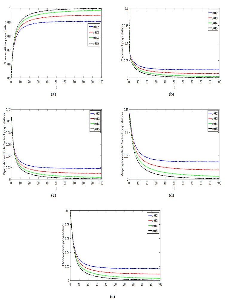
The majority of infectious illnesses, such as HIV/AIDS, Hepatitis, and coronavirus (2019-nCov), are extremely dangerous. Due to the trial version of the vaccine and different forms of 2019-nCov like beta, gamma, delta throughout the world, still, there is no control on the transmission of coronavirus. Delay factors such as social distance, quarantine, immigration limitations, holiday extensions, hospitalizations, and isolation are being utilized as essential strategies to manage the outbreak of 2019-nCov. The effect of time delay on coronavirus disease transmission is explored using a non-linear fractional order in the Caputo sense in this paper. The existence theory of the model is investigated to ensure that it has at least one and unique solution. The Ulam-Hyres (UH) stability of the considered model is demonstrated to illustrate that the stated model's solution is stable. To determine the approximate solution of the suggested model, an efficient and reliable numerical approach (Adams-Bashforth) is utilized. Simulations are used to visualize the numerical data in order to understand the behavior of the different classes of the investigated model. The effects of time delay on dynamics of coronavirus transmission are shown through numerical simulations via MATLAB-17.
- fractional derivative,
- coronavirus,
- delay model,
- Adams-Bashforth method
Citation: Lei Zhang, Mati Ur Rahman, Shabir Ahmad, Muhammad Bilal Riaz, Fahd Jarad. Dynamics of fractional order delay model of coronavirus disease[J]. AIMS Mathematics, 2022, 7(3): 4211-4232. doi: 10.3934/math.2022234

Related Papers:

Abstract

The majority of infectious illnesses, such as HIV/AIDS, Hepatitis, and coronavirus (2019-nCov), are extremely dangerous. Due to the trial version of the vaccine and different forms of 2019-nCov like beta, gamma, delta throughout the world, still, there is no control on the transmission of coronavirus. Delay factors such as social distance, quarantine, immigration limitations, holiday extensions, hospitalizations, and isolation are being utilized as essential strategies to manage the outbreak of 2019-nCov. The effect of time delay on coronavirus disease transmission is explored using a non-linear fractional order in the Caputo sense in this paper. The existence theory of the model is investigated to ensure that it has at least one and unique solution. The Ulam-Hyres (UH) stability of the considered model is demonstrated to illustrate that the stated model's solution is stable. To determine the approximate solution of the suggested model, an efficient and reliable numerical approach (Adams-Bashforth) is utilized. Simulations are used to visualize the numerical data in order to understand the behavior of the different classes of the investigated model. The effects of time delay on dynamics of coronavirus transmission are shown through numerical simulations via MATLAB-17.

References

[1]	M. D. Shereen, S. Khan, A. Kazmi, N. Bashir, R. Siddique, COVID-19 infection: Origin, transmission and characteristics of human coronaviruses, J. Adv. Res., 24 (2020), 91–98. https://doi.org/10.1016/j.jare.2020.03.005 doi: 10.1016/j.jare.2020.03.005
[2]	S. Zhao, H. Chen, Modeling the epidemic dynamics and control of COVID-19 outbreak in China, Quant. Biol., 11 (2020), 1–9. https://doi.org/10.1007/s40484-020-0199-0 doi: 10.1007/s40484-020-0199-0
[3]	E. Shim, A. Tariq, W. Choi, Y. Lee, G. Chowell, Transmission potential and severity of COVID-19 in South Korea, Int. J. Infect. Dis., 93 (2020), 339–344. https://doi.org/10.1016/j.ijid.2020.03.031 doi: 10.1016/j.ijid.2020.03.031
[4]	A. J. Kucharski, T. W. Russell, C. Diamond, Y. Liu, J. Edmunds, S. Funk, et al., Early dynamics of transmission and control of COVID-19: A mathematical modelling study, Lancet Infect. Dis., 20 (2020), 553–558. https://doi.org/10.1016/S1473-3099(20)30144-4 doi: 10.1016/S1473-3099(20)30144-4
[5]	X. Jiang, M. Coffee, A. Bari, J. Wang, X. Jiang, J. Huang, et al., Towards an artificial intelligence framework for data-driven prediction of coronavirus clinical severity, Comput. Mater. Con., 63 (2020), 537–551. https://doi.org/10.32604/cmc.2020.010691 doi: 10.32604/cmc.2020.010691
[6]	D. Fanelli, F. Piazza, Analysis and forecast of COVID-19 spreading in China, Italy and France, Chaos Soliton. Fract., 134 (2020), 109761. https://doi.org/10.1016/j.chaos.2020.109761 doi: 10.1016/j.chaos.2020.109761
[7]	A. Altan, S. Karasu, Recognition of COVID-19 disease from X-ray images by hybrid model consisting of 2D curvelet transform, chaotic salp swarm algorithm and deep learning technique, Chaos Soliton. Fract., 140 (2020), 110071. https://doi.org/10.1016/j.chaos.2020.110071 doi: 10.1016/j.chaos.2020.110071
[8]	M. Naveed, M. Rafiq, A. Raza, N. Ahmed, I. Khan, K. S. Nisar, et al., Mathematical analysis of novel coronavirus (2019-nCov) delay pandemic model, Comput. Mater. Con., 64 (2020), 1401–1414. https://doi.org/10.32604/cmc.2020.011314 doi: 10.32604/cmc.2020.011314
[9]	A. A. Kilbas, H. M. Srivastava, J. J. Trujillo, Theory and applications of fractional differential equations, Elsevier, 2006.
[10]	D. Baleanu, K. Diethelm, E. Scalas, J. J. Trujillo, Fractional calculus: Models and numerical methods, World Scientific, 2012.
[11]	D. Baleanu, J. A. T. Machado, A. C. Luo, Fractional dynamics and control, Springer Science & Business Media, 2011.
[12]	V. Lakshmikantham, S. Leela, J. V. Devi, Theory of fractional dynamic systems, Cambridge Scientific Publishers, 2009.
[13]	C. Li, D. Qian, Y. Chen, On Riemann-Liouville and caputo derivatives, Discrete Dyn. Nat. Soc., 2011 (2011), 562494. https://doi.org/10.1155/2011/562494 doi: 10.1155/2011/562494
[14]	K. S. Nisar, S. Ahmad, A. Ullah, K. Shah, H. Alrabaiah, M. Arfan, Mathematical analysis of SIRD model of COVID-19 with Caputo fractional derivative based on real data, Results Phys., 21 (2021), 103772. https://doi.org/10.1016/j.rinp.2020.103772 doi: 10.1016/j.rinp.2020.103772
[15]	I. G. Ameen, N. H. Sweilam, H. M. Ali, A fractional-order model of human liver: Analytic-approximate and numerical solutions comparing with clinical data, Alex. Eng. J., 60 (2021), 4797–4808. https://doi.org/10.1016/j.aej.2021.03.054 doi: 10.1016/j.aej.2021.03.054
[16]	S. Qureshi, A. Yusuf, A. A. Shaikh, M. Inc, D. Baleanu, Fractional modeling of blood ethanol concentration system with real data application, Chaos, 29 (2019), 013143. https://doi.org/10.1063/1.5082907 doi: 10.1063/1.5082907
[17]	F. A. Rihan, D. Baleanu, S. Lakshmanan, R. Rakkiyappan, On fractional SIRC model with salmonella bacterial infection, Abstr. Appl. Anal., 2014 (2014), 136263. https://doi.org/10.1155/2014/136263 doi: 10.1155/2014/136263
[18]	D. Baleanu, A. Jajarmi, H. Mohammadi, S. Rezapour, A new study on the mathematical modelling of human liver with Caputo-Fabrizio fractional derivative, Chaos Soliton. Fract., 134 (2020) 109705. https://doi.org/10.1016/j.chaos.2020.109705 doi: 10.1016/j.chaos.2020.109705
[19]	R. T. Alqahtani, M. A. Abdelkawy, An efficient numerical algorithm for solving fractional SIRC model with salmonella bacterial infection, Math. Biosci. Eng., 17 (2020), 3784–3793. http://www.aimspress.com/journal/MBE
[20]	R. Droghei, E. Salusti, A comparison of a fractional derivative model with an empirical model for non-linear shock waves in swelling shales, J. Petrol. Sci. Eng., 125 (2015), 181–188. https://doi.org/10.1016/j.petrol.2014.11.017 doi: 10.1016/j.petrol.2014.11.017
[21]	F. Falcini, R. Garra, A nonlocal generalization of the Exner law, J. Hydrol., 603 (2021), 126947. https://doi.org/10.1016/j.jhydrol.2021.126947 doi: 10.1016/j.jhydrol.2021.126947
[22]	R. Garra, E. Salusti, R. Droghei, Memory effects on nonlinear temperature and pressure wave propagation in the boundary between two fluid-saturated porous rocks, Adv. Math. Phys., 2015 (2015), 532150. https://doi.org/10.1155/2015/532150 doi: 10.1155/2015/532150
[23]	H. Jahanshahi, J. M. Munoz-Pacheco, S. Bekiros, N. D. Alotaibi, A fractional-order SIRD model with time-dependent memory indexes for encompassing the multi-fractional characteristics of the COVID-19, Chaos Soliton. Fract., 143 (2021), 110632. https://doi.org/10.1016/j.chaos.2020.110632 doi: 10.1016/j.chaos.2020.110632
[24]	K. Rajagopal, N. Hasanzadeh, F. Parastesh, I. I. Hamarash, S. Jafari, I. Hussain, A fractional-order model for the novel coronavirus (COVID-19) outbreak, Nonlinear Dyn., 101 (2020), 711–718. https://doi.org/10.1007/s11071-020-05757-6 doi: 10.1007/s11071-020-05757-6
[25]	S. Ahmad, A. Ullah, A. Akgül, D. Baleanu, Analysis of the fractional tumour-immune-vitamins model with Mittag-Leffler kernel, Results Phys., 19 (2020) 103559. https://doi.org/10.1016/j.rinp.2020.103559 doi: 10.1016/j.rinp.2020.103559
[26]	D. Kumar, J. Singh, D. Baleanu, On the analysis of vibration equation involving a fractional derivative with Mittag-Leffler law, Math. Method. Appl. Sci., 43 (2020), 443–457. https://doi.org/10.1002/mma.5903 doi: 10.1002/mma.5903
[27]	D. Baleanu, H. Mohammadi, S. Rezapour, A fractional differential equation model for the COVID-19 transmission by using the Caputo-Fabrizio derivative, Adv. Differ. Equ., 2020 (2020), 299. https://doi.org/10.1186/s13662-020-02762-2 doi: 10.1186/s13662-020-02762-2
[28]	S. Kumar, A. Ahmadian, R. Kumar, D. Kumar, J. Singh, D. Baleanu, et al., An efficient numerical method for fractional SIR epidemic model of infectious disease by using Bernstein wavelets, Mathematics, 8 (2020), 558. https://doi.org/10.3390/math8040558 doi: 10.3390/math8040558
[29]	J. F. Gómez-Aguilar, J. J. Rosales-García, J. J. Bernal-Alvarado, T. Córdova-Fraga, R. Guzmán-Cabrera, Fractional mechanical oscillators, Rev. mexicana de física, 58 (2012), 348–352.
[30]	K. S. Miller, B. Ross, An introduction to the fractional calculus and fractional differential equations, Willy, 1993.
[31]	H. Khan, Y. Li, A. Khan, A. Khan, Existence of solution for a fractional‐order Lotka-Volterra reaction-diffusion model with Mittag-Leffler kernel, Math. Method. Appl. Sci., 42 (2019), 3377–3387. https://doi.org/10.1002/mma.5590 doi: 10.1002/mma.5590

Reader Comments

Your name:*

Email:*
© 2022 the Author(s), licensee AIMS Press. This is an open access article distributed under the terms of the Creative Commons Attribution License (http://creativecommons.org/licenses/by/4.0)