Global attractivity for uncertain differential systems

Nana Tao; Chunxiao Ding; Nana Tao; Chunxiao Ding

doi:10.3934/math.2022122

AIMS Mathematics

2022, Volume 7, Issue 2: 2142-2159. doi: 10.3934/math.2022122

Previous Article Next Article

Research article

Global attractivity for uncertain differential systems

Nana Tao ^{1
,
,},
Chunxiao Ding ²

1.
School of Information Engineering, Kaifeng University, Kaifeng, 475004, Henan, China
2.
School of Mathematical Sciences, Liaocheng University, Liaocheng, 252059, Shandong, China

Received: 21 August 2021 Accepted: 19 October 2021 Published: 08 November 2021
MSC : 34D45, 37C75

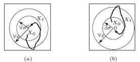
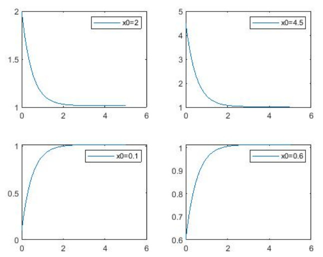
This paper studies global attractivity for uncertain differential systems, which are effective tools to solve the problems with uncertainty. And They have been applied in many areas. This article presents several global attractivity concepts. Based on the knowledge of uncertainty theory, some sufficient conditions of global attractivity for linear uncertain differential systems are given. In particular, the attractivity on the solutions and $ \alpha $-path of uncertain differential systems is studied. Last, as an application of attractivity, an interest rate model with uncertainty is shown.
- global attractivity,
- uncertain differential systems,
- sufficient condition,
- $ \alpha $-path,
- interest rate model with uncertainty
Citation: Nana Tao, Chunxiao Ding. Global attractivity for uncertain differential systems[J]. AIMS Mathematics, 2022, 7(2): 2142-2159. doi: 10.3934/math.2022122

Related Papers:

Abstract

This paper studies global attractivity for uncertain differential systems, which are effective tools to solve the problems with uncertainty. And They have been applied in many areas. This article presents several global attractivity concepts. Based on the knowledge of uncertainty theory, some sufficient conditions of global attractivity for linear uncertain differential systems are given. In particular, the attractivity on the solutions and $ \alpha $-path of uncertain differential systems is studied. Last, as an application of attractivity, an interest rate model with uncertainty is shown.

References

[1]	D. Ruelle, Characteristic exponents for a viscous fluid subjected to time dependent forces, Commun. Math. Phys., 93 (1984). doi:285–300.10.1007/BF01258529. doi: 10.1007/BF01258529
[2]	X. Yan, W. Li, Global attractivity for a class of higer order nonlinear difference equations, Appl. Math. Comput., 149 (2004), 533–546. doi: 10.1016/S0096-3003(03)00159-0. doi: 10.1016/S0096-3003(03)00159-0
[3]	K. Liu, Z. Li, Global attracting set, exponential decay and stability in distribution of neutral SPDEs driven by additive $\alpha$-stable processes, Discrete Contin. Dyn. Syst., 21 (2016), 3551–3573. doi:10.3934/dcdsb.2016110. doi: 10.3934/dcdsb.2016110
[4]	D. Xu, H. Zhao, Invariant and attracting sets of Hopfield neural networks with delay, Int. J. Syst. Sci., 32 (2002), 863–866. doi: 10.1080/002077201300306207. doi: 10.1080/002077201300306207
[5]	H. Zhao, Invariant set and attractor of nonautonomous functional differential systems, J. Math. Anal. Appl., 282 (2003), 437–443. doi: 10.1016/S0022-247X(02)00370-0. doi: 10.1016/S0022-247X(02)00370-0
[6]	D. Xu, Z. Yang, Attracting and invariant sets for a class of impulsive functional differential equations, J. Math. Anal. Appl., 329 (2007), 1036–1044. doi: 10.1016/j.jmaa.2006.05.072. doi: 10.1016/j.jmaa.2006.05.072
[7]	B. Liu, Fuzzy process, hybrid process and uncertain process, J. Uncertain Syst., 2 (2008), 3–16.
[8]	B. Liu, Uncertainty Theory: A branch of mathematics for modeling human uncertainty, Springer-Verlag, Berlin, 2010.
[9]	X. Chen, B. Liu, Existence and uniqueness theorem for uncertain differential equations, Fuzzy Optimiz. Decis. Mak., 9 (2010), 69–81. doi: 10.1007/s10700-010-9073-2. doi: 10.1007/s10700-010-9073-2
[10]	Y. Zhu, Uncertain optimal control with application to a portfolio selection model, Cybern. Syst., 41 (2010), 535-547. doi: 10.1080/01969722.2010.511552. doi: 10.1080/01969722.2010.511552
[11]	C. Ding, N. Tao, Y. Sun, Y. Zhu, The effect of time delays on transmission dynamics of schistosomiasis, Chaos, Soliton. Fract., 91 (2016), 360–371. doi: 10.1016/j.chaos.2016.06.017. doi: 10.1016/j.chaos.2016.06.017
[12]	C. Ding, Y. Sun, Y. Zhu, A NN-based hybrid intelligent algorithm for a discrete nonlinear uncertain optimal control problem, Neural. Process. Lett., (2016), doi: 10.1007/s11063-016-9536-8. doi: 10.1007/s11063-016-9536-8
[13]	J. Peng, Y. Gao, A new option pricing model for stocks in uncertainty markets, Int. J. Oper. Res., 8 (2011), 18–26. doi: http://dx.doi.org/.
[14]	X. Chen, J, Gao, Uncertain term structure model of interest rate, Soft Comput., 17 (2013), 597–604. doi: 10.1007/s00500-012-0927-0. doi: 10.1007/s00500-012-0927-0
[15]	B. Liu, Some research problems in uncertainty theory, J. Uncertain Syst., 3 (2009), 3–10. doi: 10.1007/978-3-642-01156-6. doi: 10.1007/978-3-642-01156-6
[16]	L. Deng, Y. Zhu, Existence and uniqueness theorem of solution for uncertain differential equations with jump, ICIC Expr. Lett., 6 (2012), 2693–2698.
[17]	Y. Gao, Existence and uniqueness theorems of uncertain differential equations with local Lipschitz condition, J. Uncertain Syst., 6 (2012), 223–232.
[18]	X. Ge, Y. Zhu, Existence and uniqueness theorem for uncertain delay differential equations, J. Comput. Inform. Syst., 8 (2012), 8341–8347. doi: http://dx.doi.org/.
[19]	K. Yao, H. Ke, Y. Sheng, Stability in mean for uncertain differential equation, Fuzzy Optimiz. Decis. Mak., 14 (2015), 365–379. doi: 10.1007/s10700-014-9204-2. doi: 10.1007/s10700-014-9204-2
[20]	T. Su, H. Wu, J. Zhou, Stability of multi-dimensional uncertain differential equation, Soft Comput., 20 (2016), 4991–4998. doi: 10.1007/s00500-015-1788-0. doi: 10.1007/s00500-015-1788-0
[21]	Y. Feng, X. Yang, G. Cheng, Stability in mean for multi-dimensional uncertain differential equation, Soft Comput., 22 (2018), 5783–5789. doi: 10.1007/s00500-017-2659-7. doi: 10.1007/s00500-017-2659-7
[22]	Z. Jia, X. Liu, New stability theorems of uncertain differential equations with time-dependent delay, AIMS Math., 6 (2021), 623–642. doi: 10.3934/math.2021038. doi: 10.3934/math.2021038
[23]	N. Tao, Y. Zhu, Attractivity and stability analysis of uncertain differential systems, Int. J. Bifurcat. Chaos., 25 (2015), 1550022-1-1550022-10. doi: 10.1142/S0218127415500224. doi: 10.1142/S0218127415500224
[24]	N. Tao, Y. Zhu, Stability and attractivity in optimistic value for dynamical systems with uncertainty, Int. J. Gen. Syst., 45 (2016), 418–433. doi: 10.1080/03081079.2015.1072522. doi: 10.1080/03081079.2015.1072522
[25]	B. Liu, Uncertainty Theory, 2Eds., Berlin: Springer-Verlag, 2007.
[26]	K. Yao, X. Chen, A numerical method for solving uncertain differential equations, J. Intell. Fuzzy Syst., 25 (2013), 825–832. doi: 10.3233/IFS-120688. doi: 10.3233/IFS-120688
[27]	K. Yao, Expected value of lognormal uncertain variable, Proceedings of the First International Conference on Uncertainty Theory, Urumchi, China, August 11–19, (2010), 241–243.

Reader Comments

Your name:*

Email:*
© 2022 the Author(s), licensee AIMS Press. This is an open access article distributed under the terms of the Creative Commons Attribution License (http://creativecommons.org/licenses/by/4.0)