Mathematical analysis of a fractional-order epidemic model with nonlinear incidence function

Salih Djillali; Abdon Atangana; Anwar Zeb; Choonkil Park; Salih Djillali; Abdon Atangana; Anwar Zeb; Choonkil Park

doi:10.3934/math.2022123

AIMS Mathematics

2022, Volume 7, Issue 2: 2160-2175. doi: 10.3934/math.2022123

Previous Article Next Article

Research article

Mathematical analysis of a fractional-order epidemic model with nonlinear incidence function

1.
Faculty of Exact and Computer Sciences, Mathematics Department, Hassiba Benbouali university, Chlef, Algeria
2.
Laboratoire d'Analyse Non Linéaire et Mathématiques Appliquées, University of Tlemcen, Tlemcen, Algeria
3.
Institute for Groundwater Studies, faculty of natural and agricultural science, University of the Free State, Bloemfontein, 9300, South Africa
4.
Department of Mathematics, COMSATS University Islamabad, Abbottabad Campus, Abbottabad, 22060, Khyber Pakhtunkhwa, Pakistan
5.
Research Institute for Natural Sciences, Hanyang University, Seoul 04763, Korea

Received: 16 September 2021 Accepted: 28 October 2021 Published: 08 November 2021
MSC : 49J15, 92D25, 93D20

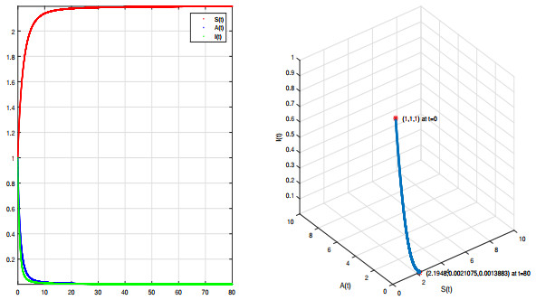
In this paper, we are interested in studying the spread of infectious disease using a fractional-order model with Caputo's fractional derivative operator. The considered model includes an infectious disease that includes two types of infected class, the first shows the presence of symptoms (symptomatic infected persons), and the second class does not show any symptoms (asymptomatic infected persons). Further, we considered a nonlinear incidence function, where it is obtained that the investigated fractional system shows some important results. In fact, different types of bifurcation are obtained, as saddle-node bifurcation, transcritical bifurcation, Hopf bifurcation, where it is discussed in detail through the research. For the numerical part, a proper numerical scheme is used for the graphical representation of the solutions. The mathematical findings are checked numerically.
- nonlinear incidence,
- bifurcation analysis,
- fractional order derivative,
- symptomatic,
- asymptomatic
Citation: Salih Djillali, Abdon Atangana, Anwar Zeb, Choonkil Park. Mathematical analysis of a fractional-order epidemic model with nonlinear incidence function[J]. AIMS Mathematics, 2022, 7(2): 2160-2175. doi: 10.3934/math.2022123

Related Papers:

Abstract

In this paper, we are interested in studying the spread of infectious disease using a fractional-order model with Caputo's fractional derivative operator. The considered model includes an infectious disease that includes two types of infected class, the first shows the presence of symptoms (symptomatic infected persons), and the second class does not show any symptoms (asymptomatic infected persons). Further, we considered a nonlinear incidence function, where it is obtained that the investigated fractional system shows some important results. In fact, different types of bifurcation are obtained, as saddle-node bifurcation, transcritical bifurcation, Hopf bifurcation, where it is discussed in detail through the research. For the numerical part, a proper numerical scheme is used for the graphical representation of the solutions. The mathematical findings are checked numerically.

References

[1]	A. Zeb, G. Zaman, S. Momani, Square-root dynamics of a giving up smoking model, Appl. Math. Model., 37 (2013), 5326–5334. doi: 10.1016/j.apm.2012.10.005.
[2]	Z. Z. Zhang, A. Zeb, S. Hussain, E. Alzahrani, Dynamics of COVID-19 mathematical model with stochastic perturbation, Adv. Differ. Equ., 2020 (2020), 451. doi: 10.1186/s13662-020-02909-1.
[3]	A. Alzahrani, A. Zeb, Detectable sensation of a stochastic smoking model, Open Math., 18 (2020), 1045–1055. doi: 10.1515/math-2020-0068.
[4]	X. Y. Zhou, J. G. Cui, Stability and Hopf bifurcation analysis of an eco-epidemiological model with delay, J. Franklin I., 347 (2010), 1654–1680. doi: 10.1016/j.jfranklin.2010.08.001.
[5]	M. A. Safi, S. M. Garba, Global stability analysis of SEIR model with holling type II incidence function, Comput. Math. Methods Med., 2012 (2012), 826052. doi: 10.1155/2012/826052.
[6]	M. A. Safi. Global stability analysis of two-stage quarantine-isolation model with Holling type II incidence function, Mathematics, 7 (2019), 350. doi: 10.3390/math7040350.
[7]	L. A. Huo, J. H. Jiang, S. X. Gong, B. He, Dynamical behavior of a rumor transmission model with Holling-type II functional response in emergency event, Physica A., 450 (2016) 228–240. doi: 10.1016/j.physa.2015.12.143.
[8]	A. Kumar, M. Kumar, Nilam, A study on the stability behavior of an epidemic model with ratio-dependent incidence and saturated treatment, Theory Biosci., 139 (2020), 225–234. doi: 10.1007/s12064-020-00314-6.
[9]	Z. A. Khan, A. L. Alaoui, A. Zeb, M. Tilioua, S. Djilali, Global dynamics of a SEI epidemic model with immigration and generalized nonlinear incidence functional, Results Phys., 27 (2021), 104477. doi: 10.1016/j.rinp.2021.104477.
[10]	A. Zeb, E. Alzahrani, V. S. Erturk, G. Zaman, Mathematical model for coronavirus disease 2019 (COVID-19) containing isolation class, Biomed. Res. Int., 2020 (2020), 3452402. doi: 10.1155/2020/3452402.
[11]	X. P. Li, H. Al Bayatti, A. Din, A. Zeb, A vigorous study of fractional order COVID-19 model via ABC derivatives, Res. Phy., 29 (2021), 104737. doi: 10.1016/j.rinp.2021.104737.
[12]	B. Soufiane, T. M. Touaoula, Global analysis of an infection age model with a class of nonlinear incidence rates, J. Math. Anal. Appl., 434 (2016), 1211–1239. doi: 10.1016/j.jmaa.2015.09.066.
[13]	M. N. Frioui, S. El-hadi Miri, T. M. Touaoula, Unified Lyapunov functional for an age-structured virus model with very general nonlinear infection response, J. Appl. Math. Comput., 58 (2018), 47–73. doi: 10.1007/s12190-017-1133-0.
[14]	I. Boudjema, T. M. Touaoula, Global stability of an infection and vaccination age-structured model with general nonlinear incidence, J. Nonlinear. Funct. Anal., 33 (2018), 1–21.
[15]	T. M. Touaoula, Global dynamics for a class of reaction-diffusion equations with distributed delay and neumann condition, Commun. Pur. Appl. Anal., 19 (2018), 2473–2490. doi: 10.3934/cpaa.2020108.
[16]	M. N. Frioui, T. M. Touaoula, B. Ainseba, Global dynamics of an age-structured model with relapse, DCDS-B, 25 (2020), 2245–2270. doi: 10.3934/dcdsb.2019226.
[17]	N. Bessonov, G. Bocharov, T. M. Touaoula, S. Trofimchuk, V. Volpert, Delay reaction-diffusion equation for infection dynamics, DCDS-B, 24 (2019), 2073–2091. doi: 10.3934/dcdsb.2019085.
[18]	T. M. Touaoula, Global stability for a class of functional differential equations (Application to Nicholson's blowflies and Mackey-Glass models), DCDS, 38 (2018), 4391–4419. doi: 10.3934/dcds.2018191.
[19]	T. M. Touaoula, M. N. Frioui, N. Bessonov, V. Volpert, Dynamics of solutions of a reaction-diffusion equation with delayed inhibition, DCDS-S, 13 (2020), 2425–2442. doi: 10.3934/dcdss.2020193.
[20]	P. Michel, T. M. Touaoula, Asymptotic behavior for a class of the renewal nonlinear equation with diffusion, Math. Method. Appl. Sci., 36 (2012), 323–335.
[21]	A. D. Bazykin, A. I. Khibnik, B. Krauskopf, Nonlinear dynamics of interacting populations, World Scientific, 1998.
[22]	X. H. Wang, Z. Wang, J. W. Xia, Stability and bifurcation control of a delayed fractional-order eco-epidemiological model with incommensurate orders, J. Franklin I., 356 (2019), 8278–8295. doi: 10.1016/j.jfranklin.2019.07.028.
[23]	J. R. Wang, M. Feckan, Y. Zhou, Nonexistence of periodic solutions and asymptotically periodic solutions for fractional differential equations, Commun. Nonlinear Sci., 18 (2013), 246–256. doi: 10.1016/j.cnsns.2012.07.004.
[24]	M. S. Asl, M. Javidi, Novel algorithms to estimate nonlinear FDEs: Applied to fractional order nutrient-phytoplankton-zooplankton system, J. Comput. Appl. Math., 339 (2018), 193-207. doi: 10.1016/j.cam.2017.10.030.
[25]	S. Bourafa, M. S. Abdelouahab, A. Moussaoui, On some extended Routh-Hurwitz conditions for fractional-order autonomous systems of order $\alpha \in$(0, 2) and their applications to some population dynamic models, Chaos Soliton. Fract., 133 (2020), 109623. doi: 10.1016/j.chaos.2020.109623.
[26]	K. Diethelm, N. J. Ford, A. D. Freed, Detailed error analysis for a fractional Adams method, Numer. Algorithms, 36 (2004), 31–52. doi: 10.1023/B:NUMA.0000027736.85078.be.
[27]	K. Diethelm, Smoothness properties of solutions of Caputo-type fractional differential equations, Fract. Calc. Appl. Anal., 10 (2007, ) 151–160.
[28]	K. P. Hadeler, P. Van den Driessche, Backward bifurcation in epidemic control, Math. Biosci., 146 (1997), 15–35. doi: 10.1016/S0025-5564(97)00027-8.
[29]	W. D. Wang, Backward bifurcation of an epidemic model with treatment, Math. Biosci., 201 (2006), 58–71. doi: 10.1016/j.mbs.2005.12.022.
[30]	B. Ghanbari, S. Djilali, Mathematical and numerical analysis of a three-species predator-prey model with herd behavior and time fractional-order derivative, Math. Method. Appl. Sci., 43 (2020), 1736–1752. doi: 10.1002/mma.5999.
[31]	B. Ghanbari, S. Djilali, Mathematical analysis of a fractional-order predator-prey model with prey social behavior and infection developed in predator population, Chaos Soliton. Fract., 138 (2020), 109960. doi: 10.1016/j.chaos.2020.109960.
[32]	S. Djilali, B. Ghanbari, The influence of an infectious disease on a prey-predator model equipped with a fractional-order derivative, Adv. Differ. Equ. 2021 (2021), 20. doi: 10.1186/s13662-020-03177-9.
[33]	S. Djilali, B. Ghanbari, Dynamical behavior of two predatorsone prey model with generalized functional response and time-fractional derivative, Adv. Differ. Equ., 2021 (2021), 235. doi: 10.1186/s13662-021-03395-9.

Reader Comments

Your name:*

Email:*
© 2022 the Author(s), licensee AIMS Press. This is an open access article distributed under the terms of the Creative Commons Attribution License (http://creativecommons.org/licenses/by/4.0)