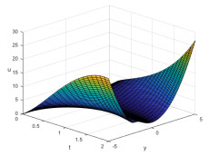
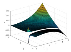
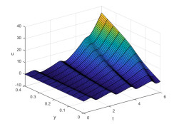
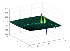
In this paper, we investigate non-traveling wave solutions of the (3+1)-dimensional variable coefficients Date-Jimbo-Kashiwara-Miwa (VC-DJKM) equation, which describes the real physical phenomena owing to the inhomogeneities of media. By combining the extended homoclinic test approach with variable separation method, we obtain abundant new exact non-traveling wave solutions of the (3+1)-dimensional VC-DJKM equation. These results with a parabolic tail or linear tail reveal the complex structure of the solutions for (3+1)-dimensional VC-DJKM equation. Moreover, the tail in these solutions maybe give a prediction of physical phenomenon. When arbitrary functions contained in these non-traveling wave solutions are taken as some special functions, we can get the kink-type solitons, singular solitary wave solutions, and periodic solitary wave solutions, and so on. As the special cases of our work, the corresponding results of (3+1)-dimensional DJKM equation, (2+1)-dimensional DJKM equation, (2+1)-dimensional VC-DJKM equation are also given.
Citation: Yuanqing Xu, Xiaoxiao Zheng, Jie Xin. New non-traveling wave solutions for (3+1)-dimensional variable coefficients Date-Jimbo-Kashiwara-Miwa equation[J]. AIMS Mathematics, 2021, 6(3): 2996-3008. doi: 10.3934/math.2021182
In this paper, we investigate non-traveling wave solutions of the (3+1)-dimensional variable coefficients Date-Jimbo-Kashiwara-Miwa (VC-DJKM) equation, which describes the real physical phenomena owing to the inhomogeneities of media. By combining the extended homoclinic test approach with variable separation method, we obtain abundant new exact non-traveling wave solutions of the (3+1)-dimensional VC-DJKM equation. These results with a parabolic tail or linear tail reveal the complex structure of the solutions for (3+1)-dimensional VC-DJKM equation. Moreover, the tail in these solutions maybe give a prediction of physical phenomenon. When arbitrary functions contained in these non-traveling wave solutions are taken as some special functions, we can get the kink-type solitons, singular solitary wave solutions, and periodic solitary wave solutions, and so on. As the special cases of our work, the corresponding results of (3+1)-dimensional DJKM equation, (2+1)-dimensional DJKM equation, (2+1)-dimensional VC-DJKM equation are also given.

| [1] | Z. Z. Lan, Periodic, breather and rogue wave solutions for a generalized (3+1)-dimensional variable-coefficient B-type Kadomtsev-Petviashvili equation in fluid dynamics, Appl. Math. Lett., 94 (2019), 126–132. |
| [2] | M. H. Huang, M. A. S. Murad, O. A. Ilhan, One-, two- and three-soliton, periodic and cross-kink solutions to the (2+1)-D variable-coefficient KP equation, Modern Phys. Lett. B, 34 (2020), 2050045. |
| [3] |
X. Y. Gao, Y. J. Guo, W. R. Shan, Magneto-optical/ferromagnetic-material computation: Bäcklund transformations, bilinear forms and N solitons for a generalized (3+1)-dimensional variable-coefficient modified Kadomtsev-Petviashvili system, Appl. Math. Lett., 111 (2021), 106627. doi: 10.1016/j.aml.2020.106627

|
| [4] |
M. Arshad, A. R. Seadawy, D. Lu, Modulation stability and optical soliton solutions of nonlinear Schrödinger equation with higher order dispersion and nonlinear terms and its applications, Superlattices Microst., 112 (2017), 422–434. doi: 10.1016/j.spmi.2017.09.054
|
| [5] |
A. R. Seadawy, K. El-Rashidy, Dispersive solitary wave solutions of Kadomtsev-Petviashvili and modified Kadomtsev-Petviashvili dynamical equations in unmagnetized dust plasma, Results Phys., 8 (2018), 1216–1222. doi: 10.1016/j.rinp.2018.01.053
|
| [6] |
Y. S. Özkan, E. Yaşar, On the exact solutions of nonlinear evolution equations by the improved tan($\varphi/2$)-expansion method, Pramana J. Phys., 94 (2020), 37. doi: 10.1007/s12043-019-1883-3
|
| [7] |
M. Iqbal, A. R. Seadawy, O. H. Khalil, D. Lu, Propagation of long internal waves in density stratified ocean for the (2+1)-dimensional nonlinear Nizhnik-Novikov-Vesselov dynamical equation, Results Phys., 16 (2020), 102838. doi: 10.1016/j.rinp.2019.102838
|
| [8] |
X. M. Peng, Y. D. Shang, X. X. Zheng, New non-travelling wave solutions of Calogero equation, Adv. Appl. Math. Mech., 8 (2016), 1036–1049. doi: 10.4208/aamm.2015.m1121
|
| [9] |
L. B. Lv, Y. D. Shang, Abundant new non-travelling wave solutions for the (3+1)-dimensional potential-YTSF equation, Appl. Math. Lett., 107 (2020), 106456. doi: 10.1016/j.aml.2020.106456
|
| [10] | J. Wang, H. L. An, B. Li, Non-traveling lump solutions and mixed lump-kink solutions to (2+1)-dimensional variable-coefficient Caudrey-Dodd-Gibbon-Kotera-Sawada equation, Modern Phys. Lett. B, 33 (2019), 1950262. |
| [11] |
S. M. Guo, L. Q. Mei, Y. B. Zhou, The compound $(G^{\prime}/G)$-expansion method and double non-traveling wave solutions of (2+1)-dimensional nonlinear partial differential equations, Comput. Math. Appl., 69 (2015), 804–816. doi: 10.1016/j.camwa.2015.02.016
|
| [12] |
J. G. Liu, Y. Tian, J. G. Hu, New non-traveling wave solutions for the (3+1)-dimensional Boiti-Leon-Manna-Pempinelli equation, Appl. Math. Lett., 79 (2018), 162–168. doi: 10.1016/j.aml.2017.12.011
|
| [13] |
A. M. Wazwaz, New (3+1)-dimensional Date-Jimbo-Kashiwara-Miwa equations with constant and time-dependent coefficients: Painlevé integrability, Phys. Lett. A, 384 (2020), 126787. doi: 10.1016/j.physleta.2020.126787
|
| [14] |
Y. Q. Yuan, B. Tian, W. R. Sun, J. Chai, L. Liu, Wronskian and Grammian solutions for a (2+1)-dimensional Date-Jimbo-Kashiwara-Miwa equation, Comput. Math. Appl., 74 (2017), 873–879. doi: 10.1016/j.camwa.2017.06.008
|
| [15] |
L. Cheng, Y. Zhang, M. J. Lin, Lax pair and lump solutions for the (2+1)-dimensional DJKM equation associated with bilinear Bäcklund transformations, Anal. Math. Phys., 9 (2019), 1741–1752. doi: 10.1007/s13324-018-0271-3
|
| [16] |
Y. H. Wang, H. Wang, C. L. Temuer, Lax pair, conservation laws, and multi-shock wave solutions of the DJKM equation with Bell polynomials and symbolic computation, Nonlinear Dynam., 78 (2014), 1101–1107. doi: 10.1007/s11071-014-1499-6
|
| [17] |
A. R. Adem, Y. Yildirim, E. Yaşar, Complexiton solutions and soliton solutions: (2+1)-dimensional Date-Jimbo-Kashiwara-Miwa equation, Pramana-J. Phys., 92 (2019), 36. doi: 10.1007/s12043-018-1707-x
|
| [18] |
Z. Z. Kang, T. C. Xia, Construction of abundant solutions of the (2+1)-dimensional time-dependent Date-Jimbo-Kashiwara-Miwa equation, Appl. Math. Lett., 103 (2020), 106163. doi: 10.1016/j.aml.2019.106163
|
| [19] |
A. M. Wazwaz, A (2+1)-dimensional time-dependent Date-Jimbo-Kashiwara-Miwa equation: Painlevé integrability and multiple soliton solutions, Comput. Math. Appl., 79 (2020), 1145–1149. doi: 10.1016/j.camwa.2019.08.025
|
Figures(8)

Yuanqing Xu, Xiaoxiao Zheng, Jie Xin. New non-traveling wave solutions for (3+1)-dimensional variable coefficients Date-Jimbo-Kashiwara-Miwa equation[J]. AIMS Mathematics, 2021, 6(3): 2996-3008. doi: 10.3934/math.2021182


 DownLoad: