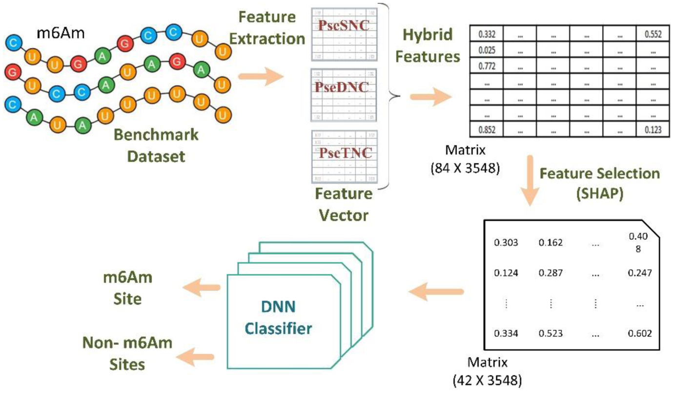
N6,2′-O-dimethyladenosine (m6Am) is a crucial RNA modification that plays a pivotal role in regulating gene expression and maintaining RNA stability. Given its dynamic involvement in various biological processes and diseases, accurately identifying m6Am is essential for understanding cellular mechanisms and pathogenesis. Furthermore, detecting m6Am modifications is key to deciphering regulatory pathways and elucidating disease mechanisms. In this study, we propose Deep-m6Am, a deep learning–based model for precisely identifying m6Am sites in RNA sequences. The proposed framework employs a comprehensive feature extraction process, i.e., integrating pseudo single nucleotide composition (PseSNC), pseudo dinucleotide composition (PseDNC), and pseudo trinucleotide composition (PseTNC) to capture complex sequence patterns. To enhance computational efficiency and eliminate noisy or redundant features, a supervised SHAP (SHapley Additive exPlanations) algorithm is utilized, ensuring the selection of the most informative features. Finally, a multilayer deep neural network (DNN) is used as a classification algorithm for identifying m6Am sites. The performance of the proposed model was evaluated in comparison with traditional machine learning (ML) algorithms and existing models. Experimental results demonstrate that Deep-m6Am outperforms previous approaches by 6.67% and traditional ML algorithms by 7.39%.
These findings highlight Deep-m6Am as a promising tool for advancing drug discovery and improving the diagnosis of diseases associated with m6Am modifications.
Citation: Islam Uddin, Salman A. AlQahtani, Sumaiya Noor, Salman Khan. Deep-m6Am: a deep learning model for identifying N6, 2′-O-Dimethyladenosine (m6Am) sites using hybrid features[J]. AIMS Bioengineering, 2025, 12(1): 145-161. doi: 10.3934/bioeng.2025006
N6,2′-O-dimethyladenosine (m6Am) is a crucial RNA modification that plays a pivotal role in regulating gene expression and maintaining RNA stability. Given its dynamic involvement in various biological processes and diseases, accurately identifying m6Am is essential for understanding cellular mechanisms and pathogenesis. Furthermore, detecting m6Am modifications is key to deciphering regulatory pathways and elucidating disease mechanisms. In this study, we propose Deep-m6Am, a deep learning–based model for precisely identifying m6Am sites in RNA sequences. The proposed framework employs a comprehensive feature extraction process, i.e., integrating pseudo single nucleotide composition (PseSNC), pseudo dinucleotide composition (PseDNC), and pseudo trinucleotide composition (PseTNC) to capture complex sequence patterns. To enhance computational efficiency and eliminate noisy or redundant features, a supervised SHAP (SHapley Additive exPlanations) algorithm is utilized, ensuring the selection of the most informative features. Finally, a multilayer deep neural network (DNN) is used as a classification algorithm for identifying m6Am sites. The performance of the proposed model was evaluated in comparison with traditional machine learning (ML) algorithms and existing models. Experimental results demonstrate that Deep-m6Am outperforms previous approaches by 6.67% and traditional ML algorithms by 7.39%.
These findings highlight Deep-m6Am as a promising tool for advancing drug discovery and improving the diagnosis of diseases associated with m6Am modifications.

| [1] |
Ye F, Wang T, Wu X, et al. (2021) N6-Methyladenosine RNA modification in cerebrospinal fluid as a novel potential diagnostic biomarker for progressive multiple sclerosis. J Transl Med 19: 1-14. https://doi.org/10.1186/S12967-021-02981-5 
|
| [2] |
Janaki Ramaiah M, Divyapriya K, Kartik Kumar S, et al. (2020) Drug-induced modifications and modulations of microRNAs and long non-coding RNAs for future therapy against glioblastoma multiforme. Gene 723: 144126. https://doi.org/10.1016/J.GENE.2019.144126
|
| [3] |
Dieterich C, Völkers M (2021) RNA modifications in cardiovascular disease—an experimental and computational perspective. Epigenetics Cardiovasc Dis 24: 113-125. https://doi.org/10.1016/B978-0-12-822258-4.00003-1
|
| [4] |
Akbar S, Khan S, Ali F, et al. (2020) iHBP-DeepPSSM: identifying hormone binding proteins using PsePSSM based evolutionary features and deep learning approach. Chemom Intell Lab Syst 204: 104103. https://doi.org/10.1016/J.CHEMOLAB.2020.104103
|
| [5] |
Chen Y, Ouyang X, Yu X, et al. (2021) N6-adenosine methylation (m6A) RNA modification: an emerging role in cardiovascular diseases. J Cardiovasc Transl Res 14: 857-872. https://doi.org/10.1007/S12265-021-10108-W
|
| [6] |
Song Z, Huang D, Song B, et al. (2021) Attention-based multi-label neural networks for integrated prediction and interpretation of twelve widely occurring RNA modifications. Nat Commun 12: 4011. https://doi.org/10.1038/s41467-021-24313-3
|
| [7] |
Jiang J, Song B, Chen K, et al. (2022) m6AmPred: identifying RNA N6, 2′-O-dimethyladenosine (m6Am) sites based on sequence-derived information. Methods 203: 328-334. https://doi.org/10.1016/J.YMETH.2021.01.007
|
| [8] |
Luo Z, Su W, Lou L, et al. (2022) DLm6Am: a deep-learning-based tool for identifying N6,2′-O-Dimethyladenosine sites in RNA sequences. Int J Mol Sci 23: 11026. https://doi.org/10.3390/ijms231911026
|
| [9] |
Jia J, Wei Z, Sun M (2023) EMDL_m6Am: identifying N6, 2′-O-dimethyladenosine sites based on stacking ensemble deep learning. BMC Bioinf 24: 397. https://doi.org/10.1186/s12859-023-05543-2
|
| [10] |
Khan S, Uddin I, Khan M, et al. (2024) Sequence based model using deep neural network and hybrid features for identification of 5-hydroxymethylcytosine modification. Sci Rep 14: 9116. https://doi.org/10.1038/s41598-024-59777-y
|
| [11] |
Khan S, Khan M, Iqbal N, et al. (2023) Enhancing sumoylation site prediction: a deep neural network with discriminative features. Life 13: 2153. https://doi.org/10.3390/life13112153
|
| [12] |
Khan S, AlQahtani SA, Noor S, et al. (2024) PSSM-Sumo: deep learning based intelligent model for prediction of sumoylation sites using discriminative features. BMC Bioinf 25: 284. https://doi.org/10.1186/s12859-024-05917-0
|
| [13] |
Uddin I, Awan HH, Khalid M, et al. (2024) A hybrid residue based sequential encoding mechanism with XGBoost improved ensemble model for identifying 5-hydroxymethylcytosine modifications. Sci Rep 14: 20819. https://doi.org/10.1038/s41598-024-71568-z
|
| [14] | Liu B, Wu H, Chou KC (2017) Pse-in-One 2.0: an improved package of web servers for generating various modes of pseudo components of DNA, RNA, and protein sequences. Nat Sci 9: 67-91. https://doi.org/10.4236/ns.2017.94007 |
| [15] |
Chen W, Lin H, Chou KC (2015) Pseudo nucleotide composition or PseKNC: an effective formulation for analyzing genomic sequences. Mol BioSyst 11: 2620-2634. https://doi.org/10.1039/c5mb00155b
|
| [16] |
Khan S, Naeem M, Qiyas M (2023) Deep intelligent predictive model for the identification of diabetes. AIMS Math 8: 16446-16462. https://doi.org/10.3934/math.2023840
|
| [17] |
Kaur G, Sharma A (2023) A deep learning-based model using hybrid feature extraction approach for consumer sentiment analysis. J Big Data 10: 1-23. https://doi.org/10.1186/S40537-022-00680-6
|
| [18] |
Gumaei A, Hassan MM, Hassan MR, et al. (2019) A hybrid feature extraction method with regularized extreme learning machine for brain tumor classification. IEEE Access 7: 36266-36273. https://doi.org/10.1109/ACCESS.2019.2904145
|
| [19] |
Noor S, Naseem A, Awan HH, et al. (2024) Deep-m5U: a deep learning-based approach for RNA 5-methyluridine modification prediction using optimized feature integration. BMC Bioinf 25: 1-23. https://doi.org/10.1186/S12859-024-05978-1
|
| [20] |
Demir S, Sahin EK (2023) An investigation of feature selection methods for soil liquefaction prediction based on tree-based ensemble algorithms using AdaBoost, Gradient boosting, and XGBoost. Neural Comput Appl 35: 3173-3190. https://doi.org/10.1007/S00521-022-07856-4
|
| [21] |
Al-Jumaili MHA, Siddique F, Abul Qais F, et al. (2023) Analysis and prediction pathways of natural products and their cytotoxicity against HeLa cell line protein using docking, molecular dynamics and ADMET. J Biomol Struct Dyn 41: 765-777. https://doi.org/10.1080/07391102.2021.2011785
|
| [22] |
Gütter J, Kruspe A, Zhu XX, et al. (2022) Impact of training set size on the ability of deep neural networks to deal with omission noise. Front Remote Sens 3: 932431. https://doi.org/10.3389/frsen.2022.932431
|
| [23] |
Chicco D, Jurman G (2023) The Matthews correlation coefficient (MCC) should replace the ROC AUC as the standard metric for assessing binary classification. BioData Min 16: 1-23. https://doi.org/10.1186/S13040-023-00322-4
|
| [24] |
Noor S, AlQahtani SA, Khan S (2025) Chronic liver disease detection using ranking and projection-based feature optimization with deep learning. AIMS Bioeng 12: 50-68. https://doi.org/10.3934/bioeng.2025003
|
| [25] | Khan S, Khan M, Iqbal N, et al. (2022) Deep-piRNA: Bi-layered prediction model for PIWI-interacting RNA using discriminative features. Comput Mater Contin 72: 2243-2258. https://doi.org/10.32604/cmc.2022.022901 |
| [26] |
Bibi N, Khan M, Khan S, et al. (2024) Sequence-based intelligent model for identification of tumor t cell antigens using fusion features. IEEE Access 12: 155040-155051. https://doi.org/10.1109/ACCESS.2024.3481244
|
| [27] |
Khan S, Khan MA, Khan M, et al. (2023) Optimized feature learning for anti-inflammatory peptide prediction using parallel distributed computing. Appl Sci 13: 7059. https://doi.org/10.3390/app13127059
|


Figures(5) / Tables(8)

Islam Uddin, Salman A. AlQahtani, Sumaiya Noor, Salman Khan. Deep-m6Am: a deep learning model for identifying N6, 2′-O-Dimethyladenosine (m6Am) sites using hybrid features[J]. AIMS Bioengineering, 2025, 12(1): 145-161. doi: 10.3934/bioeng.2025006


 DownLoad: