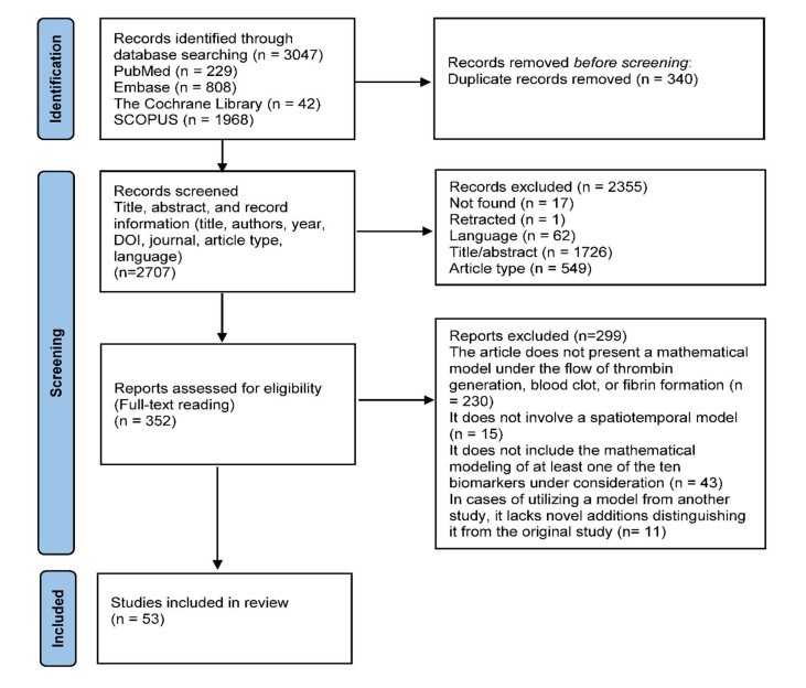
In the pursuit of personalized medicine, there is a growing demand for computational models with parameters that are easily obtainable to accelerate the development of potential solutions. Blood tests, owing to their affordability, accessibility, and routine use in healthcare, offer valuable biomarkers for assessing hemostatic balance in thrombotic and bleeding disorders. Incorporating these biomarkers into computational models of blood coagulation is crucial for creating patient-specific models, which allow for the analysis of the influence of these biomarkers on clot formation. This systematic review aims to examine how clinically relevant biomarkers are integrated into computational models of blood clot formation, thereby advancing discussions on integration methodologies, identifying current gaps, and recommending future research directions. A systematic review was conducted following the PRISMA protocol, focusing on ten clinically significant biomarkers associated with hemostatic disorders: D-dimer, fibrinogen, Von Willebrand factor, factor Ⅷ, P-selectin, prothrombin time (PT), activated partial thromboplastin time (APTT), antithrombin Ⅲ, protein C, and protein S. By utilizing this set of biomarkers, this review underscores their integration into computational models and emphasizes their integration in the context of venous thromboembolism and hemophilia. Eligibility criteria included mathematical models of thrombin generation, blood clotting, or fibrin formation under flow, incorporating at least one of these biomarkers. A total of 53 articles were included in this review. Results indicate that commonly used biomarkers such as D-dimer, PT, and APTT are rarely and superficially integrated into computational blood coagulation models. Additionally, the kinetic parameters governing the dynamics of blood clot formation demonstrated significant variability across studies, with discrepancies of up to 1, 000-fold. This review highlights a critical gap in the availability of computational models based on phenomenological or first-principles approaches that effectively incorporate affordable and routinely used clinical test results for predicting blood coagulation. This hinders the development of practical tools for clinical application, as current mathematical models often fail to consider precise, patient-specific values. This limitation is especially pronounced in patients with conditions such as hemophilia, protein C and S deficiencies, or antithrombin deficiency. Addressing these challenges by developing patient-specific models that account for kinetic variability is crucial for advancing personalized medicine in the field of hemostasis.
Citation: Mohamad Al Bannoud, Tiago Dias Martins, Silmara Aparecida de Lima Montalvão, Joyce Maria Annichino-Bizzacchi, Rubens Maciel Filho, Maria Regina Wolf Maciel. Integrating biomarkers for hemostatic disorders into computational models of blood clot formation: A systematic review[J]. Mathematical Biosciences and Engineering, 2024, 21(12): 7707-7739. doi: 10.3934/mbe.2024339
In the pursuit of personalized medicine, there is a growing demand for computational models with parameters that are easily obtainable to accelerate the development of potential solutions. Blood tests, owing to their affordability, accessibility, and routine use in healthcare, offer valuable biomarkers for assessing hemostatic balance in thrombotic and bleeding disorders. Incorporating these biomarkers into computational models of blood coagulation is crucial for creating patient-specific models, which allow for the analysis of the influence of these biomarkers on clot formation. This systematic review aims to examine how clinically relevant biomarkers are integrated into computational models of blood clot formation, thereby advancing discussions on integration methodologies, identifying current gaps, and recommending future research directions. A systematic review was conducted following the PRISMA protocol, focusing on ten clinically significant biomarkers associated with hemostatic disorders: D-dimer, fibrinogen, Von Willebrand factor, factor Ⅷ, P-selectin, prothrombin time (PT), activated partial thromboplastin time (APTT), antithrombin Ⅲ, protein C, and protein S. By utilizing this set of biomarkers, this review underscores their integration into computational models and emphasizes their integration in the context of venous thromboembolism and hemophilia. Eligibility criteria included mathematical models of thrombin generation, blood clotting, or fibrin formation under flow, incorporating at least one of these biomarkers. A total of 53 articles were included in this review. Results indicate that commonly used biomarkers such as D-dimer, PT, and APTT are rarely and superficially integrated into computational blood coagulation models. Additionally, the kinetic parameters governing the dynamics of blood clot formation demonstrated significant variability across studies, with discrepancies of up to 1, 000-fold. This review highlights a critical gap in the availability of computational models based on phenomenological or first-principles approaches that effectively incorporate affordable and routinely used clinical test results for predicting blood coagulation. This hinders the development of practical tools for clinical application, as current mathematical models often fail to consider precise, patient-specific values. This limitation is especially pronounced in patients with conditions such as hemophilia, protein C and S deficiencies, or antithrombin deficiency. Addressing these challenges by developing patient-specific models that account for kinetic variability is crucial for advancing personalized medicine in the field of hemostasis.

| [1] |
S. Z. Goldhaber, H. Bounameaux, Pulmonary embolism and deep vein thrombosis, Lancet (London, England), 379 (2012), 1835–1846. https://doi.org/10.1016/S0140-6736(11)61904-1 doi: 10.1016/S0140-6736(11)61904-1

|
| [2] |
G. E. Raskob, P. Angchaisuksiri, A. N. Blanco, H. Buller, A. Gallus, B. J. Hunt, et al., Thrombosis: a major contributor to global disease burden, Arterioscler. Thromb. Vasc. Biol., 34 (2014), 2363–2371. https://doi.org/10.1161/ATVBAHA.114.304488 doi: 10.1161/ATVBAHA.114.304488
|
| [3] |
D. Voci, U. Fedeli, I. T. Farmakis, L. Hobohm, K. Keller, L. Valerio, et al., Deaths related to pulmonary embolism and cardiovascular events before and during the 2020 COVID-19 pandemic: An epidemiological analysis of data from an Italian high-risk area, Thromb. Res., 212 (2022), 44–50. https://doi.org/10.1016/j.thromres.2022.02.008 doi: 10.1016/j.thromres.2022.02.008
|
| [4] |
I. Katsoularis, O. Fonseca-Rodríguez, P. Farrington, H. Jerndal, E. H. Lundevaller, M. Sund, et al., Risks of deep vein thrombosis, pulmonary embolism, and bleeding after covid-19: nationwide self-controlled cases series and matched cohort study, BMJ, 377 (2022). https://doi.org/10.1136/bmj-2021-069590 doi: 10.1136/bmj-2021-069590
|
| [5] |
T. N. Nguyen, M. M. Qureshi, P. Klein, H. Yamagami, M. Abdalkader, R. Mikulik, et al., Global impact of the COVID-19 pandemic on cerebral venous thrombosis and mortality, J. Stroke, 24 (2022), 256–265. https://doi.org/10.5853/jos.2022.00752 doi: 10.5853/jos.2022.00752
|
| [6] |
E. Berntorp, K. Fischer, D. P. Hart, M. E. Mancuso, D. Stephensen, A. D. Shapiro, et al., Haemophilia, Nat. Rev. Dis. Prim., 7 (2021), 45. https://doi.org/10.1038/s41572-021-00278-x doi: 10.1038/s41572-021-00278-x
|
| [7] |
K. G. Link, M. T. Stobb, M. G. Sorrells, M. Bortot, K. Ruegg, M. J. Manco‐Johnson, et al., A mathematical model of coagulation under flow identifies factor V as a modifier of thrombin generation in hemophilia A, J. Thromb. Haemost., 18 (2020), 306–317. https://doi.org/10.1111/jth.14653 doi: 10.1111/jth.14653
|
| [8] |
F. W. G. Leebeek, W. Miesbach, Gene therapy for hemophilia: a review on clinical benefit, limitations, and remaining issues, Blood, 138 (2021), 923–931. https://doi.org/10.1182/blood.2019003777 doi: 10.1182/blood.2019003777
|
| [9] |
S. S. G. Halfmann, N. Evangelatos, P. Schröder-Bäck, A. Brand, European healthcare systems readiness to shift from 'One-Size Fits All' to personalized medicine, Per. Med., 14 (2017), 63–74. https://doi.org/10.2217/pme-2016-0061 doi: 10.2217/pme-2016-0061
|
| [10] |
T. Behl, I. Kaur, A. Sehgal, S. Singh, A. Albarrati, M. Albratty, et al., The road to precision medicine: Eliminating the "One Size Fits All" approach in Alzheimer's disease, Biomed. Pharmacother., 153 (2022), 113337. https://doi.org/10.1016/j.biopha.2022.113337 doi: 10.1016/j.biopha.2022.113337
|
| [11] |
N. M. Hamdy, E. B. Basalious, M. G. El-Sisi, M. Nasr, A. M. Kabel, E. S. Nossier, et al., Advancements in current one-size-fits-all therapies compared to future treatment innovations for better improved chemotherapeutic outcomes: a step-toward personalized medicine, Curr. Med. Res. Opin., 40 (2024), 1–19. https://doi.org/10.1080/03007995.2024.2416985 doi: 10.1080/03007995.2024.2416985
|
| [12] |
G. Di Minno, E. Tremoli, Tailoring of medical treatment: hemostasis and thrombosis towards precision medicine, Haematologica, 102 (2017), 411–418. https://doi.org/10.3324/haematol.2016.156000 doi: 10.3324/haematol.2016.156000
|
| [13] | D. L. Ornstein, Chapter 41 - Personalized medicine for disorders of hemostasis and thrombosis, in Diagnostic Molecular Pathology (eds. W. B. Coleman and G. J. Tsongalis), Academic Press, (2024), 643–653. https://doi.org/10.1016/B978-0-12-822824-1.00006-7 |
| [14] |
S. Nagalla, P. F. Bray, Personalized medicine in thrombosis: back to the future, Blood, 127 (2016), 2665–2671. https://doi.org/10.1182/blood-2015-11-634832 doi: 10.1182/blood-2015-11-634832
|
| [15] |
R. J. S. Preston, J. M. O'Sullivan, Personalized approaches to the treatment of hemostatic disorders, Semin. Thromb. Hemostasis, 47 (2021), 117–119. https://doi.org/10.1055/s-0041-1723800 doi: 10.1055/s-0041-1723800
|
| [16] |
H. Al‐Samkari, W. Eng, A precision medicine approach to hereditary hemorrhagic telangiectasia and complex vascular anomalies, J. Thromb. Haemost., 20 (2022), 1077–1088. https://doi.org/10.1111/jth.15715 doi: 10.1111/jth.15715
|
| [17] |
X. Delavenne, E. Ollier, A. Lienhart, Y. Dargaud, A new paradigm for personalized prophylaxis for patients with severe haemophilia A, Haemophilia, 26 (2020), 228–235. https://doi.org/10.1111/hae.13935 doi: 10.1111/hae.13935
|
| [18] |
L. H. Bukkems, L. L. F. G. Valke, W. Barteling, B. A. P. Laros-van Gorkom, N. M. A. Blijlevens, M. H. Cnossen, et al., Combining factor Ⅷ levels and thrombin/plasmin generation: A population pharmacokinetic-pharmacodynamic model for patients with haemophilia A, Br. J. Clin. Pharmacol., 88 (2022), 2757–2768. https://doi.org/10.1111/bcp.15185 doi: 10.1111/bcp.15185
|
| [19] |
N. Mackman, W. Bergmeier, G. A. Stouffer, J. I. Weitz, Therapeutic strategies for thrombosis: new targets and approaches, Nat. Rev. Drug. Discov., 19 (2020), 333–352. https://doi.org/10.1038/s41573-020-0061-0 doi: 10.1038/s41573-020-0061-0
|
| [20] |
P. S. Wells, R. Ihaddadene, A. Reilly, M. A. Forgie, Diagnosis of venous thromboembolism: 20 years of progress, Ann. Intern. Med., 168 (2018), 131–140. https://doi.org/10.7326/M17-0291 doi: 10.7326/M17-0291
|
| [21] |
F. Khan, T. Tritschler, S. R. Kahn, M. A. Rodger, Venous thromboembolism, Lancet (London, England), 398 (2021), 64–77. https://doi.org/10.1016/S0140-6736(20)32658-1 doi: 10.1016/S0140-6736(20)32658-1
|
| [22] |
T. D. Martins, S. D. Martins, S. Montalvão, M. Al Bannoud, G. Y. Ottaiano, L. Q. Silva, et al., Combining artificial neural networks and hematological data to diagnose Covid-19 infection in Brazilian population, Neural Comput. Appl., 36 (2024), 4387–4399. https://doi.org/10.1007/s00521-023-09312-3 doi: 10.1007/s00521-023-09312-3
|
| [23] |
T. D. Martins, R. Maciel-Filho, S. A. L. Montalvão, G. S. S. Gois, M. Al Bannoud, G. Y. Ottaiano, et al., Predicting mortality of cancer patients using artificial intelligence, patient data and blood tests, Neural Comput. Appl., 36 (2024), 15599–15616. https://doi.org/10.1007/s00521-024-09915-4 doi: 10.1007/s00521-024-09915-4
|
| [24] |
F. W. G. Leebeek, New developments in diagnosis and management of acquired hemophilia and acquired von willebrand syndrome, HemaSphere, 5 (2021). https://doi.org/10.1097/HS9.0000000000000586 doi: 10.1097/HS9.0000000000000586
|
| [25] |
F. Peyvandi, G. Kenet, I. Pekrul, R. K. Pruthi, P. Ramge, M. Spannagl, Laboratory testing in hemophilia: Impact of factor and non‐factor replacement therapy on coagulation assays, J. Thromb. Haemost., 18 (2020), 1242–1255. https://doi.org/10.1111/jth.14784 doi: 10.1111/jth.14784
|
| [26] |
B. Pezeshkpoor, J. Oldenburg, A. Pavlova, Insights into the molecular genetic of hemophilia A and hemophilia B: The relevance of genetic testing in routine clinical practice, Hamostaseologie, 42 (2022), 390–399. https://doi.org/10.1055/a-1945-9429 doi: 10.1055/a-1945-9429
|
| [27] |
A. H. Kristoffersen, E. Ajzner, D. Rogic, E. Y. Sozmen, P. Carraro, A. P. Faria, et al., Is D-dimer used according to clinical algorithms in the diagnostic work-up of patients with suspicion of venous thromboembolism? A study in six European countries, Thromb. Res., 142 (2016), 1–7. https://doi.org/10.1016/j.thromres.2016.04.001 doi: 10.1016/j.thromres.2016.04.001
|
| [28] |
M. Kafeza, J. Shalhoub, N. Salooja, L. Bingham, K. Spagou, A. H. Davies, A systematic review of clinical prediction scores for deep vein thrombosis, Phlebology, 32 (2017), 516–531. https://doi.org/10.1177/0268355516678729 doi: 10.1177/0268355516678729
|
| [29] |
M. T. Greene, A. C. Spyropoulos, V. Chopra, P. J. Grant, S. Kaatz, S. J. Bernstein, et al., Validation of risk assessment models of venous thromboembolism in hospitalized medical patients, Am. J. Med., 129 (2016), 1001.e9–1001.e18. https://doi.org/10.1016/j.amjmed.2016.03.031 doi: 10.1016/j.amjmed.2016.03.031
|
| [30] |
P. C. Silveira, I. K. Ip, S. Z. Goldhaber, G. Piazza, C. B. Benson, R. Khorasani, Performance of wells score for deep vein thrombosis in the inpatient setting, JAMA Intern. Med., 175 (2015), 1112–1117. https://doi.org/10.1001/jamainternmed.2015.1687 doi: 10.1001/jamainternmed.2015.1687
|
| [31] |
M. Kafeza, J. Shalhoub, N. Salooja, L. Bingham, K. Spagou, A. H. Davies, A systematic review of clinical prediction scores for deep vein thrombosis, Phlebology, 32 (2016), 516–531. https://doi.org/10.1177/0268355516678729 doi: 10.1177/0268355516678729
|
| [32] |
I. Nichele, A. Tosetto, Scoring Systems for Estimating the Risk of Recurrent Venous Thromboembolism, Semin. Thromb. Hemost., 43 (2017), 493–499. https://doi.org/10.1055/s-0037-1602662 doi: 10.1055/s-0037-1602662
|
| [33] |
A. Muñoz, C. Ay, E. Grilz, S. López, C. Font, V. Pachón, et al., A clinical-genetic risk score for predicting cancer-associated venous thromboembolism: A development and validation study involving two independent prospective cohorts, J. Clin. Oncol., 41 (2023), 2911–2925. https://doi.org/10.1200/JCO.22.00255 doi: 10.1200/JCO.22.00255
|
| [34] |
F. Rodeghiero, A. Tosetto, T. Abshire, D. M. Arnold, B. Coller, P. James, et al., ISTH/SSC bleeding assessment tool: a standardized questionnaire and a proposal for a new bleeding score for inherited bleeding disorders, J. Thromb. Haemost., 8 (2010), 2063–2065. https://doi.org/10.1111/j.1538-7836.2010.03975.x doi: 10.1111/j.1538-7836.2010.03975.x
|
| [35] |
M. Borhany, N. Fatima, M. Abid, T. Shamsi, M. Othman, Application of the ISTH bleeding score in hemophilia, Transfus. Apher. Sci., 57 (2018), 556–560. https://doi.org/10.1016/j.transci.2018.06.003 doi: 10.1016/j.transci.2018.06.003
|
| [36] |
M. Khalifa, M. Albadawy, Artificial intelligence for clinical prediction: Exploring key domains and essential functions, Comput. Methods Programs Biomed. Updat., 5 (2024), 100148. https://doi.org/10.1016/j.cmpbup.2024.100148 doi: 10.1016/j.cmpbup.2024.100148
|
| [37] |
T. H. Tan, C. C. Hsu, C. J. Chen, S. L. Hsu, T. L. Liu, H. J. Lin, et al., Predicting outcomes in older ED patients with influenza in real time using a big data-driven and machine learning approach to the hospital information system, BMC Geriatr., 21 (2021), 280. https://doi.org/10.1186/s12877-021-02229-3 doi: 10.1186/s12877-021-02229-3
|
| [38] |
C. Guan, F. Ma, S. Chang, J. Zhang, Interpretable machine learning models for predicting venous thromboembolism in the intensive care unit: an analysis based on data from 207 centers, Crit. Care, 27 (2023), 406. https://doi.org/10.1186/s13054-023-04683-4 doi: 10.1186/s13054-023-04683-4
|
| [39] |
T. D. Martins, J. M. Annichino-Bizzacchi, A. V. C. Romano, R. Maciel Filho, Artificial neural networks for prediction of recurrent venous thromboembolism, Int. J. Med. Inform., 141 (2020), 104221. https://doi.org/10.1016/j.ijmedinf.2020.104221 doi: 10.1016/j.ijmedinf.2020.104221
|
| [40] |
I. Pabinger, C. Ay, Biomarkers and venous thromboembolism, Arter. Thromb. Vasc. Biol., 29 (2009), 332–336. https://doi.org/10.1161/ATVBAHA.108.182188 doi: 10.1161/ATVBAHA.108.182188
|
| [41] |
I. Pabinger, J. Thaler, C. Ay, Biomarkers for prediction of venous thromboembolism in cancer, Blood, 122 (2013), 2011–2018. https://doi.org/10.1182/blood-2013-04-460147 doi: 10.1182/blood-2013-04-460147
|
| [42] |
F. Galeano-Valle, L. Ordieres-Ortega, C. M. Oblitas, J. del-Toro-Cervera, L. Alvarez-Sala-Walther, P. Demelo-Rodríguez, Inflammatory biomarkers in the short-term prognosis of venous thromboembolism: A narrative review, Int. J. Mol. Sci., 22 (2021), 2627. https://doi.org/10.3390/ijms22052627 doi: 10.3390/ijms22052627
|
| [43] |
B. Jacobs, A. Obi, T. Wakefield, Diagnostic biomarkers in venous thromboembolic disease, J. Vasc. Surg. Venous Lymphat. Disord., 4 (2016), 508–517. https://doi.org/10.1016/j.jvsv.2016.02.005 doi: 10.1016/j.jvsv.2016.02.005
|
| [44] |
M. A. Bannoud, B. P. Gomes, M. C. de S. P. Abdalla, M. V Freire, K. Andreola, T. D. Martins, et al., Mathematical modeling of drying kinetics of ground Açaí (Euterpe oleracea) kernel using artificial neural networks, Chem. Pap., 78 (2024), 1033–1054. https://doi.org/10.1007/s11696-023-03142-2 doi: 10.1007/s11696-023-03142-2
|
| [45] |
M. A. Bannoud, T. D. Martins, B. F. dos Santos, Control of a closed dry grinding circuit with ball mills using predictive control based on neural networks, Digit. Chem. Eng., 5 (2022), 100064. https://doi.org/10.1016/j.dche.2022.100064 doi: 10.1016/j.dche.2022.100064
|
| [46] |
J. Berg, K. Nyström, Data-driven discovery of PDEs in complex datasets, J. Comput. Phys., 384 (2019), 239–252. https://doi.org/10.1016/j.jcp.2019.01.036 doi: 10.1016/j.jcp.2019.01.036
|
| [47] |
L. Burzawa, L. Li, X. Wang, A. Buganza-Tepole, D. M. Umulis, Acceleration of PDE-based biological simulation through the development of neural network metamodels, Curr. Pathobiol. Rep., 8 (2020), 121–131. https://doi.org/10.1007/s40139-020-00216-8 doi: 10.1007/s40139-020-00216-8
|
| [48] |
M. A. Bannoud, C. A. M. da Silva, T. D. Martins, Applications of metaheuristic optimization algorithms in model predictive control for chemical engineering processes: A systematic review, Annu. Rev. Control., 58 (2024), 100973. https://doi.org/10.1016/j.arcontrol.2024.100973 doi: 10.1016/j.arcontrol.2024.100973
|
| [49] |
M. A. Bannoud, P. H. N. Ferreira, R. R. de Andrade, C. A. M. da Silva, Control of an integrated first and second-generation continuous alcoholic fermentation process with cell recycling using model predictive control, Chem. Eng. Commun., (2024), 1–24. https://doi.org/10.1080/00986445.2024.2417901 doi: 10.1080/00986445.2024.2417901
|
| [50] |
Y. Zhao, C. Li, X. Liu, R. Qian, R. Song, X. Chen, Patient-specific seizure prediction via adder network and supervised contrastive learning, IEEE Trans. Neural Syst. Rehabil. Eng., 30 (2022), 1536–1547. https://doi.org/10.1109/TNSRE.2022.3180155 doi: 10.1109/TNSRE.2022.3180155
|
| [51] |
K. Leiderman, S. S. Sindi, D. M. Monroe, A. L. Fogelson, K. B. Neeves, The art and science of building a computational model to understand hemostasis, Semin. Thromb. Hemost., 47 (2021), 129–138. https://doi.org/10.1055/s-0041-1722861 doi: 10.1055/s-0041-1722861
|
| [52] |
N. Ratto, A. Bouchnita, P. Chelle, M. Marion, M. Panteleev, D. Nechipurenko, et al., Patient-specific modelling of blood coagulation, Bull. Math. Biol., 83 (2021), 50. https://doi.org/10.1007/s11538-021-00890-8 doi: 10.1007/s11538-021-00890-8
|
| [53] |
R. Burghaus, K. Coboeken, T. Gaub, L. Kuepfer, A. Sensse, H.-U. Siegmund, et al., Evaluation of the efficacy and safety of rivaroxaban using a computer model for blood coagulation, PLoS One, 6 (2011), e17626. https://doi.org/10.1371/journal.pone.0017626 doi: 10.1371/journal.pone.0017626
|
| [54] |
C. Watson, H. Saaid, V. Vedula, J. C. Cardenas, P. K. Henke, F. Nicoud, et al., Venous thromboembolism: Review of clinical challenges, biology, assessment, treatment, and modeling, Ann. Biomed. Eng., 52 (2024), 467–486. https://doi.org/10.1007/s10439-023-03390-z doi: 10.1007/s10439-023-03390-z
|
| [55] |
N. N. Ramli, S. Iberahim, N. H. M. Noor, Z. Zulkafli, T. M. T. M. Shihabuddin, M. H. Din, et al., Haemostasis and inflammatory parameters as potential diagnostic biomarkers for VTE in trauma-immobilized patients, Diagnostics (Basel), 13 (2023), 150. https://doi.org/10.3390/diagnostics13010150 doi: 10.3390/diagnostics13010150
|
| [56] |
L. G. R. Ferreira, R. C. Figueiredo, M. das Graças Carvalho, D. R. A. Rios, Thrombin generation assay as a biomarker of cardiovascular outcomes and mortality: A narrative review, Thromb. Res., 220 (2022), 107–115. https://doi.org/10.1016/j.thromres.2022.10.007 doi: 10.1016/j.thromres.2022.10.007
|
| [57] |
M. S. Edvardsen, K. Hindberg, E. S. Hansen, V. M. Morelli, T. Ueland, P. Aukrust, et al., Plasma levels of von Willebrand factor and future risk of incident venous thromboembolism, Blood Adv., 5 (2021), 224–232. https://doi.org/10.1182/bloodadvances.2020003135 doi: 10.1182/bloodadvances.2020003135
|
| [58] |
L. Anghel, R. Sascău, R. Radu, C. Stătescu, From classical laboratory parameters to novel biomarkers for the diagnosis of venous thrombosis, Int. J. Mol. Sci., 21 (2020), 1920. https://doi.org/10.3390/ijms21061920 doi: 10.3390/ijms21061920
|
| [59] |
H. Y. Lim, C. O'Malley, G. Donnan, H. Nandurkar, P. Ho, A review of global coagulation assays — Is there a role in thrombosis risk prediction?, Thromb. Res., 179 (2019), 45–55. https://doi.org/10.1016/j.thromres.2019.04.033 doi: 10.1016/j.thromres.2019.04.033
|
| [60] |
H. Hou, Z. Ge, P. Ying, J. Dai, D. Shi, Z. Xu, et al., Biomarkers of deep venous thrombosis, J. Thromb. Thrombolysis., 34 (2012), 335–346. https://doi.org/10.1007/s11239-012-0721-y doi: 10.1007/s11239-012-0721-y
|
| [61] |
D. Moher, A. Liberati, J. Tetzlaff, D. G. Altman, Preferred reporting items for systematic reviews and meta-analyses: the PRISMA statement, PLoS Med., 6 (2009), e1000097. https://doi.org/10.1371/journal.pmed.1000097 doi: 10.1371/journal.pmed.1000097
|
| [62] |
M. J. Page, J. E. McKenzie, P. M. Bossuyt, I. Boutron, T. C. Hoffmann, C. D. Mulrow, et al., The PRISMA 2020 statement: an updated guideline for reporting systematic reviews, BMJ, 372 (2021), n71. https://doi.org/10.1136/bmj.n71 doi: 10.1136/bmj.n71
|
| [63] |
E. N. Sorensen, G. W. Burgreen, W. R. Wagner, J. F. Antaki, Computational simulation of platelet deposition and activation: I. Model development and properties, Ann. Biomed. Eng., 27 (1999), 436–448. https://doi.org/10.1114/1.200 doi: 10.1114/1.200
|
| [64] |
K. Boryczko, W. Dzwinel, D. A. Yuen, Modeling fibrin aggregation in blood flow with discrete-particles, Comput. Methods Programs Biomed., 75 (2004), 181–194. https://doi.org/10.1016/j.cmpb.2004.02.001 doi: 10.1016/j.cmpb.2004.02.001
|
| [65] |
I. V. Pivkin, P. D. Richardson, G. Karniadakis, Blood flow velocity effects and role of activation delay time on growth and form of platelet thrombi, Proc. Natl. Acad. Sci. USA, 103 (2006), 17164–17169. https://doi.org/10.1073/pnas.0608546103 doi: 10.1073/pnas.0608546103
|
| [66] |
Z. Xu, N. Chen, M. M. Kamocka, E. D. Rosen, M. Alber, A multiscale model of thrombus development, J. R. Soc. Interface, 5 (2008), 705–722. https://doi.org/10.1098/rsif.2007.1202 doi: 10.1098/rsif.2007.1202
|
| [67] |
Z. Xu, N. Chen, S. C. Shadden, J. E. Marsden, M. M. Kamocka, E. D. Rosen, et al., Study of blood flow impact on growth of thrombi using a multiscale model, Soft. Matter, 5 (2009), 769–779. https://doi.org/10.1039/B812429A doi: 10.1039/B812429A
|
| [68] |
Z. Xu, J. Lioi, J. Mu, M. M. Kamocka, X. Liu, D. Z. Chen, et al., A multiscale model of venous thrombus formation with surface-mediated control of blood coagulation cascade, Biophys. J., 98 (2010), 1723–1732. https://doi.org/10.1016/j.bpj.2009.12.4331 doi: 10.1016/j.bpj.2009.12.4331
|
| [69] |
A. M. Shibeko, E. S. Lobanova, M. A. Panteleev, F. I. Ataullakhanov, Blood flow controls coagulation onset via the positive feedback of factor Ⅶ activation by factor Xa, BMC Syst. Biol., 4 (2010), 5. https://doi.org/10.1186/1752-0509-4-5 doi: 10.1186/1752-0509-4-5
|
| [70] |
S. W. Jordan, E. L. Chaikof, Simulated surface-induced thrombin generation in a flow field, Biophys. J., 101 (2011), 276–286. https://doi.org/10.1016/j.bpj.2011.05.056 doi: 10.1016/j.bpj.2011.05.056
|
| [71] |
K. Leiderman, A. L. Fogelson, Grow with the flow: a spatial-temporal model of platelet deposition and blood coagulation under flow, Math. Med. Biol., 28 (2011), 47–84. https://doi.org/10.1093/imammb/dqq005 doi: 10.1093/imammb/dqq005
|
| [72] |
A. L. Fogelson, Y. H. Hussain, K. Leiderman, Blood clot formation under flow: The importance of factor XI depends strongly on platelet count, Biophys. J., 102 (2012), 10–18. https://doi.org/10.1016/j.bpj.2011.10.048 doi: 10.1016/j.bpj.2011.10.048
|
| [73] |
K. Leiderman, A. L. Fogelson, The influence of hindered transport on the development of platelet thrombi under flow, Bull. Math. Biol., 75 (2013), 1255–1283. https://doi.org/10.1007/s11538-012-9784-3 doi: 10.1007/s11538-012-9784-3
|
| [74] |
A. Tosenberger, F. Ataullakhanov, N. Bessonov, M. Panteleev, A. Tokarev, V. Volpert, Modelling of thrombus growth in flow with a DPD-PDE method, J. Theor. Biol., 337 (2013), 30–41. https://doi.org/10.1016/j.jtbi.2013.07.023 doi: 10.1016/j.jtbi.2013.07.023
|
| [75] |
A. Sequeira, T. Bodnár, Blood coagulation simulations using a viscoelastic model, Math. Model. Nat. Phenom., 9 (2014), 34–45. https://doi.org/10.1051/mmnp/20149604 doi: 10.1051/mmnp/20149604
|
| [76] |
A. Tosenberger, N. Bessonov, V. Volpert, Influence of fibrinogen deficiency on clot formation in flow by hybrid model, Math. Model. Nat. Phenom., 10 (2015), 36–47. https://doi.org/10.1051/mmnp/201510102 doi: 10.1051/mmnp/201510102
|
| [77] |
O. S. Rukhlenko, O. A. Dudchenko, K. E. Zlobina, G. T. Guria, Mathematical modeling of intravascular blood coagulation under wall shear stress, PLoS One, 10 (2015), e0134028. https://doi.org/10.1371/journal.pone.0134028 doi: 10.1371/journal.pone.0134028
|
| [78] |
J. Pavlova, A. Fasano, J. Janela, A. Sequeira, Numerical validation of a synthetic cell-based model of blood coagulation, J. Theor. Biol., 380 (2015), 367–379. https://doi.org/10.1016/j.jtbi.2015.06.004 doi: 10.1016/j.jtbi.2015.06.004
|
| [79] |
A. Piebalgs, X. Y. Xu, Towards a multi-physics modelling framework for thrombolysis under the influence of blood flow, J. R. Soc. Interface, 12 (2015), 20150949. https://doi.org/10.1098/rsif.2015.0949 doi: 10.1098/rsif.2015.0949
|
| [80] |
Z. Li, A. Yazdani, A. Tartakovsky, G. E. Karniadakis, Transport dissipative particle dynamics model for mesoscopic advection-diffusion-reaction problems, J. Chem. Phys., 143 (2015), 14101. https://doi.org/10.1063/1.4923254 doi: 10.1063/1.4923254
|
| [81] |
A. Bouchnita, K. Bouzaachane, T. Galochkina, P. Kurbatova, P. Nony, V. Volpert, An individualized blood coagulation model to predict INR therapeutic range during warfarin treatment, Math. Model. Nat. Phenom., 11 (2016), 28–44. https://doi.org/10.1051/mmnp/201611603 doi: 10.1051/mmnp/201611603
|
| [82] |
J. H. Seo, T. Abd, R. T. George, R. Mittal, A coupled chemo-fluidic computational model for thrombogenesis in infarcted left ventricles, Am. J. Physiol. Heart Circ. Physiol., 310 (2016), H1567–82. https://doi.org/10.1152/ajpheart.00855.2015 doi: 10.1152/ajpheart.00855.2015
|
| [83] |
M. N. Ngoepe, Y. Ventikos, Computational modelling of clot development in patient-specific cerebral aneurysm cases, J. Thromb. Haemost., 14 (2016), 262–272. https://doi.org/10.1111/jth.13220 doi: 10.1111/jth.13220
|
| [84] |
A. Bouchnita, T. Galochkina, V. Volpert, Influence of antithrombin on the regimes of blood coagulation: Insights from the mathematical model, Acta Biotheor., 64 (2016), 327–342. https://doi.org/10.1007/s10441-016-9291-2 doi: 10.1007/s10441-016-9291-2
|
| [85] |
E. V. Dydek, E. L. Chaikof, Simulated thrombin generation in the presence of surface-bound heparin and circulating tissue factor, Ann. Biomed. Eng., 44 (2016), 1072–1084. https://doi.org/10.1007/s10439-015-1377-5 doi: 10.1007/s10439-015-1377-5
|
| [86] |
J. Pavlova, A. Fasano, A. Sequeira, Numerical simulations of a reduced model for blood coagulation, Zeitschrift für Angew. Math. und Phys., 67 (2016), 28. https://doi.org/10.1007/s00033-015-0610-2 doi: 10.1007/s00033-015-0610-2
|
| [87] |
A. Tosenberger, F. Ataullakhanov, N. Bessonov, M. Panteleev, A. Tokarev, V. Volpert, Modelling of platelet-fibrin clot formation in flow with a DPD-PDE method, J. Math. Biol., 72 (2016), 649–681. https://doi.org/10.1007/s00285-015-0891-2 doi: 10.1007/s00285-015-0891-2
|
| [88] |
V. Govindarajan, V. Rakesh, J. Reifman, A. Y. Mitrophanov, Computational study of thrombus formation and clotting factor effects under venous flow conditions, Biophys. J., 110 (2016), 1869–1885. https://doi.org/10.1016/j.bpj.2016.03.010 doi: 10.1016/j.bpj.2016.03.010
|
| [89] |
C. Ou, W. Huang, M. M.-F. Yuen, A computational model based on fibrin accumulation for the prediction of stasis thrombosis following flow-diverting treatment in cerebral aneurysms, Med. Biol. Eng. Comput., 55 (2017), 89–99. https://doi.org/10.1007/s11517-016-1501-1 doi: 10.1007/s11517-016-1501-1
|
| [90] |
A. Yazdani, H. Li, J. D. Humphrey, G. E. Karniadakis, A general shear-dependent model for thrombus formation, PLoS Comput. Biol., 13 (2017), e1005291. https://doi.org/10.1371/journal.pcbi.1005291 doi: 10.1371/journal.pcbi.1005291
|
| [91] |
H. Hosseinzadegan, D. K. Tafti, Prediction of thrombus growth: Effect of stenosis and reynolds number, Cardiovasc. Eng. Technol., 8 (2017), 164–181. https://doi.org/10.1007/s13239-017-0304-3 doi: 10.1007/s13239-017-0304-3
|
| [92] |
L. M. Haynes, T. Orfeo, K. G. Mann, S. J. Everse, K. E. Brummel-Ziedins, Probing the dynamics of clot-bound thrombin at venous shear rates, Biophys. J., 112 (2017), 1634–1644. https://doi.org/10.1016/j.bpj.2017.03.002 doi: 10.1016/j.bpj.2017.03.002
|
| [93] |
H. Kamada, Y. Imai, M. Nakamura, T. Ishikawa, T. Yamaguchi, Shear-induced platelet aggregation and distribution of thrombogenesis at stenotic vessels, Microcirculation, 24 (2017). https://doi.org/10.1111/micc.12355 doi: 10.1111/micc.12355
|
| [94] |
J. D. Horn, D. J. Maitland, J. Hartman, J. M. Ortega, A computational thrombus formation model: application to an idealized two-dimensional aneurysm treated with bare metal coils, Biomech. Model. Mechanobiol., 17 (2018), 1821–1838. https://doi.org/10.1007/s10237-018-1059-y doi: 10.1007/s10237-018-1059-y
|
| [95] |
R. Méndez Rojano, S. Mendez, F. Nicoud, Introducing the pro-coagulant contact system in the numerical assessment of device-related thrombosis, Biomech. Model. Mechanobiol., 17 (2018), 815–826. https://doi.org/10.1007/s10237-017-0994-3 doi: 10.1007/s10237-017-0994-3
|
| [96] |
B. Gu, A. Piebalgs, Y. Huang, C. Longstaff, A. D. Hughes, R. Chen, et al., Mathematical modelling of intravenous thrombolysis in acute ischaemic stroke: Effects of dose regimens on levels of fibrinolytic proteins and clot lysis time, Pharmaceutics, 11 (2019), 111. https://doi.org/10.3390/pharmaceutics11030111 doi: 10.3390/pharmaceutics11030111
|
| [97] |
K. Ayabe, S. Goto, H. Oka, H. Yabushita, M. Nakayama, A. Tomita, et al., Potential different impact of inhibition of thrombin function and thrombin generation rate for the growth of thrombi formed at site of endothelial injury under blood flow condition, Thromb. Res., 179 (2019), 121–127. https://doi.org/10.1016/j.thromres.2019.05.007 doi: 10.1016/j.thromres.2019.05.007
|
| [98] |
J. Chen, S. L. Diamond, Reduced model to predict thrombin and fibrin during thrombosis on collagen/tissue factor under venous flow: Roles of γ'-fibrin and factor XIa, PLoS Comput. Biol., 15 (2019), e1007266. https://doi.org/10.1371/journal.pcbi.1007266 doi: 10.1371/journal.pcbi.1007266
|
| [99] |
A. Bouchnita, V. Volpert, A multiscale model of platelet-fibrin thrombus growth in the flow, Comput. Fluids, 184 (2019), 10–20. https://doi.org/10.1016/j.compfluid.2019.03.021 doi: 10.1016/j.compfluid.2019.03.021
|
| [100] |
H. Hosseinzadegan, D. K. Tafti, A predictive model of thrombus growth in stenosed vessels with dynamic geometries, J. Med. Biol. Eng., 39 (2019), 605–621. https://doi.org/10.1007/s40846-018-0443-5 doi: 10.1007/s40846-018-0443-5
|
| [101] |
O. E. Kadri, V. D. Chandran, M. Surblyte, R. S. Voronov, In vivo measurement of blood clot mechanics from computational fluid dynamics based on intravital microscopy images, Comput. Biol. Med., 106 (2019), 1–11. https://doi.org/10.1016/j.compbiomed.2019.01.001 doi: 10.1016/j.compbiomed.2019.01.001
|
| [102] |
J. Du, D. Kim, G. Alhawael, D. N. Ku, A. L. Fogelson, Clot permeability, agonist transport, and platelet binding kinetics in arterial thrombosis, Biophys. J., 119 (2020), 2102–2115. https://doi.org/10.1016/j.bpj.2020.08.041 doi: 10.1016/j.bpj.2020.08.041
|
| [103] |
W. T. Wu, M. Zhussupbekov, N. Aubry, J. F. Antaki, M. Massoudi, Simulation of thrombosis in a stenotic microchannel: The effects of vWF-enhanced shear activation of platelets, Int. J. Eng. Sci., 147 (2020), 103206. https://doi.org/10.1016/j.ijengsci.2019.103206 doi: 10.1016/j.ijengsci.2019.103206
|
| [104] |
A. Bouchnita, K. Terekhov, P. Nony, Y. Vassilevski, V. Volpert, A mathematical model to quantify the effects of platelet count, shear rate, and injury size on the initiation of blood coagulation under venous flow conditions, PLoS One, 15 (2020), e0235392. https://doi.org/10.1371/journal.pone.0235392 doi: 10.1371/journal.pone.0235392
|
| [105] |
Z. L. Liu, D. N. Ku, C. K. Aidun, Mechanobiology of shear-induced platelet aggregation leading to occlusive arterial thrombosis: A multiscale in silico analysis, J. Biomech., 120 (2021), 110349. https://doi.org/10.1016/j.jbiomech.2021.110349 doi: 10.1016/j.jbiomech.2021.110349
|
| [106] |
V. N. Kaneva, J. L. Dunster, V. Volpert, F. Ataullahanov, M. A. Panteleev, D. Y. Nechipurenko, Modeling thrombus shell: Linking adhesion receptor properties and macroscopic dynamics, Biophys. J., 120 (2021), 334–351. https://doi.org/10.1016/j.bpj.2020.10.049 doi: 10.1016/j.bpj.2020.10.049
|
| [107] |
A. Yazdani, Y. Deng, H. Li, E. Javadi, Z. Li, S. Jamali, et al., Integrating blood cell mechanics, platelet adhesive dynamics and coagulation cascade for modelling thrombus formation in normal and diabetic blood, J. R. Soc. Interface., 18 (2021), 20200834. https://doi.org/10.1098/rsif.2020.0834 doi: 10.1098/rsif.2020.0834
|
| [108] |
C. Ma, Y. Ren, Q. Zheng, J. Wang, A computational model on cartesian adaptive grid for thrombosis simulation, IEEE Access, 10 (2022), 67694–67702. https://doi.org/10.1109/ACCESS.2022.3184123 doi: 10.1109/ACCESS.2022.3184123
|
| [109] |
R. Méndez Rojano, A. Lai, M. Zhussupbekov, G. W. Burgreen, K. Cook, J. F. Antaki, A fibrin enhanced thrombosis model for medical devices operating at low shear regimes or large surface areas, PLoS Comput. Biol., 18 (2022), e1010277. https://doi.org/10.1371/journal.pcbi.1010277 doi: 10.1371/journal.pcbi.1010277
|
| [110] |
M. Rezaeimoghaddam, F. N. van de Vosse, Continuum modeling of thrombus formation and growth under different shear rates, J. Biomech., 132 (2022), 110915. https://doi.org/10.1016/j.jbiomech.2021.110915 doi: 10.1016/j.jbiomech.2021.110915
|
| [111] | A. S. Pisaryuk, N. M. Povalyaev, A. V Poletaev, A. M. Shibeko, Systems biology approach for personalized hemostasis correction, J. Pers. Med., 12 (2022). https://doi.org/10.3390/jpm12111903 |
| [112] |
M. Zhussupbekov, R. Méndez Rojano, W. T. Wu, J. F. Antaki, von Willebrand factor unfolding mediates platelet deposition in a model of high-shear thrombosis, Biophys. J., 121 (2022), 4033–4047. https://doi.org/10.1016/j.bpj.2022.09.040 doi: 10.1016/j.bpj.2022.09.040
|
| [113] |
Y. Wang, J. Luan, K. Luo, T. Zhu, J. Fan, Multi-constituent simulation of thrombosis in aortic dissection, Int. J. Eng. Sci., 184 (2023), 103817. http://dx.doi.org/10.1016/j.ijengsci.2023.103817 doi: 10.1016/j.ijengsci.2023.103817
|
| [114] |
R. Petkantchin, A. Rousseau, O. Eker, K. Zouaoui Boudjeltia, F. Raynaud, B. Chopard, A simplified mesoscale 3D model for characterizing fibrinolysis under flow conditions, Sci. Rep., 13 (2023), 13681. https://doi.org/10.1038/s41598-023-40973-1 doi: 10.1038/s41598-023-40973-1
|
| [115] |
K. Miyazawa, A. L. Fogelson, K. Leiderman, Inhibition of platelet-surface-bound proteins during coagulation under flow Ⅱ: Antithrombin and heparin, Biophys. J., 122 (2023), 230–240. https://doi.org/10.1016/j.bpj.2022.10.038 doi: 10.1016/j.bpj.2022.10.038
|
| [116] |
A. R. Rezaie, S. T. Olson, Calcium enhances heparin catalysis of the antithrombin-factor Xa reaction by promoting the assembly of an intermediate heparin-antithrombin-factor Xa bridging complex: Demonstration by rapid kinetics studies, Biochemistry, 39 (2000), 12083–12090. https://doi.org/10.1021/bi0011126 doi: 10.1021/bi0011126
|
| [117] |
M. Anand, K. Rajagopal, K. R. Rajagopal, A model for the formation, growth, and lysis of clots in quiescent plasma: A comparison between the effects of antithrombin Ⅲ deficiency and protein C deficiency, J. Theor. Biol., 253 (2008), 725–738. https://doi.org/10.1016/j.jtbi.2008.04.015 doi: 10.1016/j.jtbi.2008.04.015
|
| [118] | M. J. Griffith, The heparin-enhanced antithrombin Ⅲ/thrombin reaction is saturable with respect to both thrombin and antithrombin Ⅲ, J. Biol. Chem., 257 (1982), 13302–13899. |
| [119] | M. J. Griffith, Kinetics of the heparin-enhanced antithrombin Ⅲ/thrombin reaction. Evidence for a template model for the mechanism of action of heparin, J. Biol. Chem., 257 (1982), 7360–7365. |
| [120] |
C. M. Danforth, T. Orfeo, K. G. Mann, K. E. Brummel-Ziedins, S. J. Everse, The impact of uncertainty in a blood coagulation model, Math. Med. Biol., 26 (2009), 323–336. https://doi.org/10.1093/imammb/dqp011 doi: 10.1093/imammb/dqp011
|
| [121] |
P. P. Naidu, M. Anand, Importance of Ⅷa inactivation in a mathematical model for the formation, growth, and lysis of clots, Math. Model. Nat. Phenom., 9 (2014), 17–33. https://doi.org/10.1051/mmnp/20149603 doi: 10.1051/mmnp/20149603
|
| [122] |
F. Saitta, J. Masuri, M. Signorelli, S. Bertini, A. Bisio, D. Fessas, Thermodynamic insights on the effects of low-molecular-weight heparins on antithrombin Ⅲ, Thermochim. Acta, 713 (2022), 179248. https://doi.org/10.1016/j.tca.2022.179248 doi: 10.1016/j.tca.2022.179248
|
| [123] |
H. Minakami, M. Morikawa, T. Yamada, T. Yamada, Candidates for the determination of antithrombin activity in pregnant women, J. Perinat. Med., 39 (2011), 369–374. https://doi.org/10.1515/jpm.2011.026 doi: 10.1515/jpm.2011.026
|
| [124] | K. C. Jones, K. G. Mann, A model for the tissue factor pathway to thrombin. Ⅱ: A mathematical simulation, J. Biol. Chem., 269 (1994), 23367–23373. |
| [125] |
M. F. Hockin, K. C. Jones, S. J. Everse, K. G. Mann, A model for the stoichiometric regulation of blood coagulation, J. Biol. Chem., 277 (2002), 18322–18333. https://doi.org/10.1074/jbc.m201173200 doi: 10.1074/jbc.m201173200
|
| [126] |
R. Méndez Rojano, S. Mendez, D. Lucor, A. Ranc, M. Giansily-Blaizot, J. F. Schved, et al., Kinetics of the coagulation cascade including the contact activation system: sensitivity analysis and model reduction, Biomech. Model. Mechanobiol., 18 (2019), 1139–1153. https://doi.org/10.1007/s10237-019-01134-4 doi: 10.1007/s10237-019-01134-4
|
| [127] |
M. S. Chatterjee, W. S. Denney, H. Jing, S. L. Diamond, Systems biology of coagulation initiation: Kinetics of thrombin generation in resting and activated human blood, PLOS Comput. Biol., 6 (2010), e1000950. https://doi.org/10.1371/journal.pcbi.1000950 doi: 10.1371/journal.pcbi.1000950
|
| [128] |
A. Ranc, S. Bru, S. Mendez, M. Giansily-Blaizot, F. Nicoud, R. Méndez Rojano, Critical evaluation of kinetic schemes for coagulation, PLoS One, 18 (2023), e0290531. https://doi.org/10.1371/journal.pone.0290531 doi: 10.1371/journal.pone.0290531
|
| [129] |
M. F. Hockin, K. C. Jones, S. J. Everse, K. G. Mann, A model for the stoichiometric regulation of blood coagulation, J. Biol. Chem., 277 (2002), 18322–18333. https://doi.org/10.1074/jbc.m201173200 doi: 10.1074/jbc.m201173200
|
| [130] |
D. Luan, M. Zai, J. D. Varner, Computationally derived points of fragility of a human cascade are consistent with current therapeutic strategies, PLoS Comput. Biol., 3 (2007), 1347–1359. https://doi.org/10.1371/journal.pcbi.0030142 doi: 10.1371/journal.pcbi.0030142
|
| [131] |
K. G. Link, M. T. Stobb, J. Di Paola, K. B. Neeves, A. L. Fogelson, S. S. Sindi, et al., A local and global sensitivity analysis of a mathematical model of coagulation and platelet deposition under flow, PLoS One, 13 (2018), e0200917. https://doi.org/10.1371/journal.pone.0200917 doi: 10.1371/journal.pone.0200917
|
 mbe-21-12-339 supplementary.pdf mbe-21-12-339 supplementary.pdf |
 |

Figures(2) / Tables(3)

Mohamad Al Bannoud, Tiago Dias Martins, Silmara Aparecida de Lima Montalvão, Joyce Maria Annichino-Bizzacchi, Rubens Maciel Filho, Maria Regina Wolf Maciel. Integrating biomarkers for hemostatic disorders into computational models of blood clot formation: A systematic review[J]. Mathematical Biosciences and Engineering, 2024, 21(12): 7707-7739. doi: 10.3934/mbe.2024339


 DownLoad: