Volatility, a pivotal factor in the financial stock market, encapsulates the dynamic nature of asset prices and reflects both instability and risk. A volatility quantitative investment strategy is a methodology that utilizes information about volatility to guide investors in trading and profit-making. With the goal of enhancing the effectiveness and robustness of investment strategies, our methodology involved three prominent time series models with six machine learning models: K-nearest neighbors, AdaBoost, CatBoost, LightGBM, XGBoost, and random forest, which meticulously captured the intricate patterns within historical volatility data. These models synergistically combined to create eighteen novel fusion models to predict volatility with precision. By integrating the forecasting results with quantitative investing principles, we constructed a new strategy that achieved better returns in twelve selected American financial stocks. For investors navigating the real stock market, our findings serve as a valuable reference, potentially securing an average annualized return of approximately 5 to 10% for the American financial stocks under scrutiny in our research.
Citation: Keyue Yan, Ying Li. Machine learning-based analysis of volatility quantitative investment strategies for American financial stocks[J]. Quantitative Finance and Economics, 2024, 8(2): 364-386. doi: 10.3934/QFE.2024014
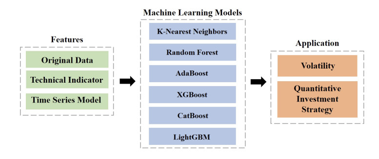
Volatility, a pivotal factor in the financial stock market, encapsulates the dynamic nature of asset prices and reflects both instability and risk. A volatility quantitative investment strategy is a methodology that utilizes information about volatility to guide investors in trading and profit-making. With the goal of enhancing the effectiveness and robustness of investment strategies, our methodology involved three prominent time series models with six machine learning models: K-nearest neighbors, AdaBoost, CatBoost, LightGBM, XGBoost, and random forest, which meticulously captured the intricate patterns within historical volatility data. These models synergistically combined to create eighteen novel fusion models to predict volatility with precision. By integrating the forecasting results with quantitative investing principles, we constructed a new strategy that achieved better returns in twelve selected American financial stocks. For investors navigating the real stock market, our findings serve as a valuable reference, potentially securing an average annualized return of approximately 5 to 10% for the American financial stocks under scrutiny in our research.

| [1] |
Alsulmi M, Al-Shahrani N (2022) Machine Learning-Based Decision-Making for Stock Trading: Case Study for Automated Trading in Saudi Stock Exchange. Sci Program, 6542862. https://doi.org/10.1155/2022/6542862 doi: 10.1155/2022/6542862

|
| [2] | Attanasio G, Cagliero L, Garza P, et al. (2019) Quantitative cryptocurrency trading: exploring the use of machine learning techniques. 5th Workshop on Data Science for Macro-modeling with Financial and Economic Datasets, 1–6. https://doi.org/10.1145/3336499.3338003 |
| [3] |
Ayyildiz N, Iskenderoglu O (2024) How effective is machine learning in stock market predictions? Heliyon 10: 1–10. https://doi.org/10.1016/j.heliyon.2024.e24123 doi: 10.1016/j.heliyon.2024.e24123
|
| [4] |
Basak S, Kar S, Saha S, et al. (2019) Predicting the direction of stock market prices using tree-based classifiers. N Am J Econ Financ 47: 552–567. https://doi.org/10.1016/j.najef.2018.06.013 doi: 10.1016/j.najef.2018.06.013
|
| [5] |
Bezerra PCS, Albuquerque PHM (2017) Volatility forecasting via SVR–GARCH with mixture of Gaussian kernels. Comput Manag Sci 14: 179–196. https://doi.org/10.1007/s10287-016-0267-0 doi: 10.1007/s10287-016-0267-0
|
| [6] |
Brooks C, Persand G (2003) Volatility forecasting for risk management. J Forecast 22: 1–22. https://doi.org/10.1002/for.841 doi: 10.1002/for.841
|
| [7] |
Diane L, Brijlal P (2024) Forecasting Stock Market Realized Volatility using Random Forest and Artificial Neural Network in South Africa. Int J Econ Financ Iss 14: 5–14. https://doi.org/10.32479/ijefi.15431 doi: 10.32479/ijefi.15431
|
| [8] |
Epaphra M (2016) Modeling exchange rate volatility: Application of the GARCH and EGARCH models. J Math Financ 7: 121–143. https://doi.org/10.4236/jmf.2017.71007 doi: 10.4236/jmf.2017.71007
|
| [9] |
Gao Y, Wang R, Zhou E (2021) Stock prediction based on optimized LSTM and GRU models. Sci Program, 1–8. https://doi.org/10.1155/2021/4055281 doi: 10.1155/2021/4055281
|
| [10] |
Herwartz H (2017) Stock return prediction under GARCH—An empirical assessment. Int J Forecast 33: 569–580. https://doi.org/10.1016/j.ijforecast.2017.01.002 doi: 10.1016/j.ijforecast.2017.01.002
|
| [11] | Karasan A (2021) Machine Learning for Financial Risk Management with Python. O'Reilly. |
| [12] |
Khan W, Ghazanfar MA, Azam MA, et al. (2020) Stock market prediction using machine learning classifiers and social media, news. J Amb Intel Hum Comp 13: 3433–3456. https://doi.org/10.1007/s12652-020-01839-w doi: 10.1007/s12652-020-01839-w
|
| [13] |
Khand S, Anand V, Qureshi MN, et al. (2019) The performance of exponential moving average, moving average convergence-divergence, relative strength index and momentum trading rules in the Pakistan stock market. Indian J Sci Technol 12: 1–22. https://doi.org/10.17485/ijst/2019/v12i26/145117 doi: 10.17485/ijst/2019/v12i26/145117
|
| [14] | Khanderwal S, Mohanty D (2021) Stock price prediction using ARIMA model. In J Market Hum Resource Res 2: 98–107. |
| [15] |
Kumbure MM, Lohrmann C, Luukka P, et al. (2022) Machine learning techniques and data for stock market forecasting: A literature review. Expert Syst Appl 197: 116659. https://doi.org/10.1016/j.eswa.2022.116659 doi: 10.1016/j.eswa.2022.116659
|
| [16] | Lai CY, Chen RC, Caraka RE (2019) Prediction stock price based on different index factors using LSTM. 2019 International conference on machine learning and cybernetics (ICMLC), 1–6. https://doi.org/10.1109/icmlc48188.2019.8949162 |
| [17] |
Levy RA (1967) Relative strength as a criterion for investment selection. J Financ 22: 595–610. https://doi.org/10.2307/2326004 doi: 10.2307/2326004
|
| [18] |
Li Y, Yan K (2023) Prediction of Barrier Option Price Based on Antithetic Monte Carlo and Machine Learning Methods. Cloud Comput Data Sci 4: 77–86. https://doi.org/10.37256/ccds.4120232110 doi: 10.37256/ccds.4120232110
|
| [19] |
Lo HC, Chan CY(2023) Mean reverting in stock ratings distribution. Rev Quantit Financ Account 60: 1065–1097. https://doi.org/10.1007/s11156-022-01121-4 doi: 10.1007/s11156-022-01121-4
|
| [20] |
Luong C, Dokuchaev N (2018) Forecasting of realised volatility with the random forests algorithm. J Risk Financ Manage 11: 61. https://doi.org/10.3390/jrfm11040061 doi: 10.3390/jrfm11040061
|
| [21] |
Monfared SA, Enke D (2014) Volatility forecasting using a hybrid GJR-GARCH neural network model. Procedia Comput Sci 36: 246–253. https://doi.org/10.1016/j.procs.2014.09.087 doi: 10.1016/j.procs.2014.09.087
|
| [22] | Müller AC, Guido S (2016) Introduction to machine learning with Python: a guide for data scientists. O'Reilly Media. |
| [23] |
Nikou M, Mansourfar G, Bagherzadeh J (2019) Stock price prediction using DEEP learning algorithm and its comparison with machine learning algorithms. Intel Syst Account Financ Manage 26: 164–174. https://doi.org/10.1002/isaf.1459 doi: 10.1002/isaf.1459
|
| [24] |
Nti IK, Adekoya AF, Weyori BA (2020) A systematic review of fundamental and technical analysis of stock market predictions. Artif Intell Rev 53: 3007–3057. https://doi.org/10.1007/s10462-019-09754-z doi: 10.1007/s10462-019-09754-z
|
| [25] |
Patel J, Shah S, Thakkar P, et al. (2015) Predicting stock and stock price index movement using trend deterministic data preparation and machine learning techniques. Expert Syst Appl 42: 259–268. https://doi.org/10.1016/j.eswa.2014.07.040 doi: 10.1016/j.eswa.2014.07.040
|
| [26] |
Rezaei H, Faaljou H, Mansourfar G (2021) Stock price prediction using deep learning and frequency decomposition. Expert Syst Appl 169: 114332. https://doi.org/10.1016/j.eswa.2020.114332 doi: 10.1016/j.eswa.2020.114332
|
| [27] |
Rouf N, Malik MB, Arif T, Sharma S, et al. (2021) Stock market prediction using machine learning techniques: a decade survey on methodologies, recent developments, and future directions. Electronics 10: 2717. https://doi.org/10.3390/electronics10212717 doi: 10.3390/electronics10212717
|
| [28] |
Schwert GW (1990) Stock market volatility. Financ Anal J 46: 23–34. https://doi.org/10.2469/faj.v46.n3.23 doi: 10.2469/faj.v46.n3.23
|
| [29] |
Shahi TB, Shrestha A, Neupane A, et al. (2020) Stock price forecasting with deep learning: A comparative study. Mathematics 8: 1441. https://doi.org/10.3390/math8091441 doi: 10.3390/math8091441
|
| [30] |
Sun H, Yu B (2020) Forecasting financial returns volatility: a GARCH-SVR model. Comput Econ 55: 451–471. https://doi.org/10.1007/s10614-019-09896-w doi: 10.1007/s10614-019-09896-w
|
| [31] | Tatsat H, Puri S, Lookabaugh B (2020) Machine Learning and Data Science Blueprints for Finance. O'Reilly Media. |
| [32] |
Vijh M, Chandola D, Tikkiwal VA, et al. (2020) Stock closing price prediction using machine learning techniques. Procedia Comput Sci 167: 599–606. https://doi.org/10.1016/j.procs.2020.03.326 doi: 10.1016/j.procs.2020.03.326
|
| [33] |
Wang J, Kim J (2018) Predicting stock price trend using MACD optimized by historical volatility. Math Probl Eng 2018: 1–12. https://doi.org/10.1155/2018/9280590 doi: 10.1155/2018/9280590
|
| [34] | Wang Y, Yan K (2022) Prediction of Significant Bitcoin Price Changes Based on Deep Learning. 5th International Conference on Data Science and Information Technology (DSIT 2022), 1–5. https://doi.org/10.1109/dsit55514.2022.9943971 |
| [35] |
Wang Y, Yan K (2023) Machine learning-based quantitative trading strategies across different time intervals in the American market. Quant Financ Econ 7: 569–594. https://doi.org/10.3934/qfe.2023028 doi: 10.3934/qfe.2023028
|
| [36] | Yahoo Finance (2024) Available from: https://finance.yahoo.com/. |
| [37] |
Yan K, Wang N, Li Y (2024) Research on Double Fusion Modeling for Volatility Quantitative Trading Strategies in Hong Kong Stock Market. Finance 14: 844–855. https://doi.org/10.12677/fin.2024.143090 doi: 10.12677/fin.2024.143090
|
| [38] | Yan K, Wang Y (2023) Prediction of Bitcoin prices' trends with ensemble learning models. 5th International Conference on Computer Information Science and Artificial Intelligence (CISAI 2022), 900–905. https://doi.org/10.1117/12.2667793 |
| [39] |
Yan K, Wang Y, Li Y (2023) Enhanced Bollinger Band Stock Quantitative Trading Strategy Based on Random Forest. Art Intell Evolution 4: 22–33. https://doi.org/10.37256/aie.4120231991 doi: 10.37256/aie.4120231991
|
| [40] |
Yu P, Yan X (2020) Stock price prediction based on deep neural networks. Neural Comput Appl 32: 1609–1628. https://doi.org/10.1007/s00521-019-04212-x doi: 10.1007/s00521-019-04212-x
|
| [41] |
Zhang YJ, Zhang H (2023) Volatility forecasting of crude oil market: which structural change based GARCH models have better performance? Energ J 44: 175–194. https://doi.org/10.5547/ej44-1-Zhang doi: 10.5547/ej44-1-Zhang
|


Figures(8) / Tables(7)

Keyue Yan, Ying Li. Machine learning-based analysis of volatility quantitative investment strategies for American financial stocks[J]. Quantitative Finance and Economics, 2024, 8(2): 364-386. doi: 10.3934/QFE.2024014


 DownLoad: