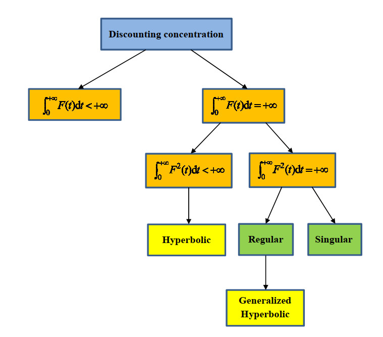
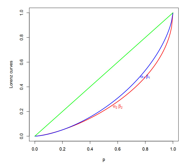
The framework of this paper was intertemporal choice, that is to say, the process whereby people were required to choose between a smaller-sooner reward and a larger-later income. In this study, the selection of rewards was supported by a discount function instead of direct preferences between the involved rewards. The objective of this paper was to measure the discounting concentration of a discount function through a variant of the Gini index and the Lorenz curve usually used in statistics. Both measures allowed for the comparison of the discounting concentration corresponding to two discount functions. The methodology employed in this paper was based on the parallelism between a discount function and the distribution function of an absolutely continuous random variable. This similarity allowed us to export the measures of concentration from the field of statistics to finance. The main result of this work was the analysis of the discounting concentration depending on other characteristics of the shape of a discount function (regularity and super-additivity) and the total area under the discount function curve.
Citation: Salvador Cruz Rambaud, Piedad Ortiz Fernández, Javier Sánchez García, Paula Ortega Perals. A proposal of concentration measures for discount functions[J]. Quantitative Finance and Economics, 2024, 8(2): 347-363. doi: 10.3934/QFE.2024013
The framework of this paper was intertemporal choice, that is to say, the process whereby people were required to choose between a smaller-sooner reward and a larger-later income. In this study, the selection of rewards was supported by a discount function instead of direct preferences between the involved rewards. The objective of this paper was to measure the discounting concentration of a discount function through a variant of the Gini index and the Lorenz curve usually used in statistics. Both measures allowed for the comparison of the discounting concentration corresponding to two discount functions. The methodology employed in this paper was based on the parallelism between a discount function and the distribution function of an absolutely continuous random variable. This similarity allowed us to export the measures of concentration from the field of statistics to finance. The main result of this work was the analysis of the discounting concentration depending on other characteristics of the shape of a discount function (regularity and super-additivity) and the total area under the discount function curve.

| [1] |
Atkinson T (1970) On the measurement of inequality. J Econ Theory 2: 244–263. https://doi.org/10.1016/0022-0531(70)90039-6 doi: 10.1016/0022-0531(70)90039-6

|
| [2] |
Bonetti M, Gigliarano C, Muliere P (2009) The Gini concentration test for survival data. Lifetime Data Anal 15: 493–518. https://doi.org/10.1007/s10985-009-9125-5 doi: 10.1007/s10985-009-9125-5
|
| [3] |
Caliendo FN, Findley TS (2014) Discount functions and self-control problems. Econ Lett 122: 416–419. https://doi.org/10.2139/ssrn.2337093 doi: 10.2139/ssrn.2337093
|
| [4] | Calot G (1965) Cours de Statistique Descriptive. Dunod, Paris. |
| [5] |
Chambers CP, Echenique F, Miller AD (2023) Decreasing Impatience. Am Econ J Microecon 15: 527–551. https://doi.org/10.1257/mic.20210361 doi: 10.1257/mic.20210361
|
| [6] | Cramér H (1961) Mathematical Methods of Statistics, Asia Publishing House, Bombay. |
| [7] |
Cruz Rambaud S (2014) A new argument in favor of hyperbolic discounting in very long term project appraisal. Int J Theoretical Appl Financ 17: 1450049. https://doi.org/10.1142/S0219024914500496 doi: 10.1142/S0219024914500496
|
| [8] | Cruz Rambaud S, González Fernández I, Ventre V (2018) Modeling the inconsistency in intertemporal choice: The generalized Weibull discount function and its extension. Ann Financ 14: 415–426. |
| [9] |
Gastwirth JL (1971) A general definition of the Lorenz curve. Econometrica 39: 1037–1039. https://doi.org/10.2307/1909675 doi: 10.2307/1909675
|
| [10] | Kotz S (2006) Encyclopedia of Statistical Sciences (Second Edition). Wiley-Interscience, Hoboken (New Jersey). |
| [11] | Lubrano M (2017) The econometrics of inequality and poverty. Lecture 4: Lorenz curves, the Gini coefficient and parametric distributions. Available from: https://citeseerx.ist.psu.edu/viewdoc/download?doi=10.1.1.169.4809&rep=rep1&type=pdf. |
| [12] | Lueddeckens S, Saling P, Guenther E (2022) Discounting and life cycle assessment: A distorting measure in assessments, a reasonable instrument for decisions. Int J Environ Sci Technol 19: 2961–-2972. |
| [13] | Sarabia JM (2008) Parametric Lorenz curves: Models and applications, In: Chotikapanich, D., editor, Modeling Income Distributions and Lorenz Curves, volume 5 of Economic Studies in Equality, Social Exclusion and Well-Being, Chapter 9, 167–190. Springer, New York. https://link.springer.com/chapter/10.1007/978-0-387-72796-7_9 |
| [14] | Shaked M, Shanthikumar JG (1994) Stochastic Orders and Their Applications, Boston: Academic Press, Inc. |
| [15] |
Takeuchi K (2011) Non-parametric test of time consistency: Present bias and future bias. Game Econ Behav 71: 456–478. https://doi.org/10.1016/j.geb.2010.05.005 doi: 10.1016/j.geb.2010.05.005
|
| [16] |
Zhou C, Tang W, Zhao R (2015) Optimal consumer search with prospect utility in hybrid uncertain environment. J Uncertain Anal Appl 3, 6. https://doi.org/10.1186/s40467-015-0030-z doi: 10.1186/s40467-015-0030-z
|
Figures(4) / Tables(2)

Salvador Cruz Rambaud, Piedad Ortiz Fernández, Javier Sánchez García, Paula Ortega Perals. A proposal of concentration measures for discount functions[J]. Quantitative Finance and Economics, 2024, 8(2): 347-363. doi: 10.3934/QFE.2024013


 DownLoad: