Dynamics and numerical simulations of a generalized mosquito-borne epidemic model using the Ornstein-Uhlenbeck process: Stability, stationary distribution, and probability density function

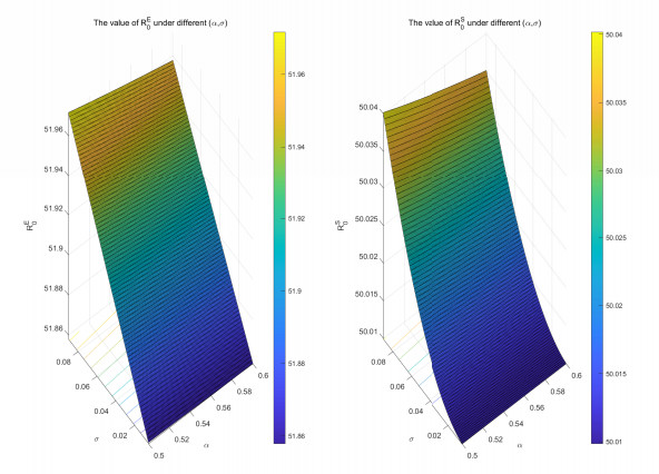
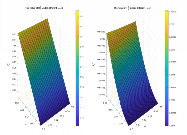
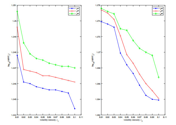
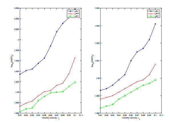
1.   Introduction

Mosquito-borne infectious diseases, a common type of vector-borne infections diseases, are primarily caused by pathogens, which are transmitted from mosquitoes to humans or other animals ^[1]. Mosquitoes are one of the most widely distributed vectors in the world, transmitting a variety of parasites and viruses. While the vector organisms may not develop the disease themselves, they serve as a means for the pathogen to spread among hosts. With mosquitoes found in various locations from tropical to temperate zones, mosquito-borne infections have a wide and diverse geographic distribution ^[2]. Diseases such as malaria, lymphatic filariasis, West Nile Virus, Zika virus, and dengue fever are commonly transmitted by mosquitoes, with no specific vaccine or medication available for treatment. These diseases pose a significant threat to human health and socio-economic development worldwide.

Malaria is an infectious disease caused by a protozoan parasite that is mainly transmitted to humans through the bite of a mosquito ^[3]. The disease is widespread in tropical and subtropical regions, particularly in poorer areas of Africa, Asia, and Latin America. Globally, malaria remains a major public health problem, resulting in millions of infections and hundreds of thousands of deaths annually. Apart from malaria, as the classic mosquito-borne infectious disease, dengue fever also attracts considerable attention. Dengue fever is a serious infectious disease caused by the dengue virus, primarily transmitted to humans by the Aedes aegypti mosquito, but also through blood transfusion, organ transplantation, and vertical transmission ^[4]. In addition, both yellow fever and West Nile disease are also caused by mosquitoes carrying the corresponding viral infections ^[5,6]. Yellow fever is a rare disease among U.S. travelers. Conversely, West Nile virus is the primary mosquito-borne disease in the continental U.S., commonly transmitted through the bite of an infected mosquito.

Research on mosquito-borne diseases has proliferated ^[7,8,9,10]. Mathematical models have been increasingly used for experimental and observational studies of different biological phenomena, and a wide range of techniques and applications have been developed to study epidemic diseases. For example, Newton and Reiter ^[8] developed a deterministic Susceptibility, Exposure, Infection, Resistance, and Removal (SEIR) model of dengue transmission to explore the behavior of epidemics and realistically reproduce epidemic transmission in immunologically unmade populations. Moreover, Pandey et al. ^[9] proposed a Caputo fractional order derivative mathematical model of dengue disease to study the transmission dynamics of the disease and to make reliable conclusions about the behavior of dengue epidemics. In addition, in order to investigate the effect of the vector on the dynamics of the disease, Shi and Zhao et al. ^[10] proposed a differential system with saturated incidence to model a vector-borne disease

the biological significance of the model (1.1) parameters are shown in Table 1. In this model, there are two populations, namely mosquito vector population and human host population. The mosquito vector population is divided into two categories, $S_V$ and $I_V$, and $N = S_V+I_V$, while human host population is divided into three categories, $S_H, I_H$ and $R_H$. According to ^[10], it is reasonable to assume that the total number of human $K = S_H+I_H+R_H$ is a positive constant.

Obviously, we can get that there always exists a compact positively invariant set for model (1.1) as follows

The incidence rate has various forms and plays an important role in the study of epidemic dynamics. In addition to the saturated incidence used in model ($1.1$) of this paper, other forms of the incidence rate have been widely used. For example, Chong, Tchuenche, and Smith ^[11] studied a mathematical model of avian influenza with half-saturated incidence rate $\frac{S_bI_b}{H_b+I_b}$, $\frac{S_HI_a}{H_a+I_a}$ and $\frac{S_hI_m}{H_m+I_m}$. In addition, Li et al. ^[12] also carried out numerical analysis of friteral order pine wilt disease model with bilinear incidence rate $S_hI_v$ and $I_hS_v$. In order to make the model ($1.1$) have wider research significance and apply to more infectious diseases, we consider replacing the saturated incidence rate with the general incidence rate $\phi_1(I_V)$, $\phi_2(I_H)$ and $\phi_3(I_H)$, and then give the epidemic model with the general incidence as follows

Furthermore, the incidence rate in model (1.3) are assumed to meet the following conditions

$(\mathcal{A}_1)\ \phi_1(0) = \phi_2(0) = \phi_3(0) = 0$,

$(\mathcal{A}_2)\ \phi_1^{'}(I_V) \geq 0, \phi_2^{'}(I_H) \geq 0, \phi_3^{'}(I_H) \geq 0, \forall \ I_V, I_H \geq 0$,

$(\mathcal{A}_3)\ 0\leq(\frac{I_V}{\phi_1(I_V)})^{'} \leq m_0, 0\leq(\frac{I_H}{\phi_2(I_H)})^{'} \leq m_0, 0\leq(\frac{I_H}{\phi_3(I_H)})^{'} \leq m_0$, where $m_0$ is a positive constant.

By looking at the model (1.3), the following equation is valid, $\frac{dN}{dt} = \Lambda-mN$, that indicates, $N(t) \rightarrow \frac{\Lambda}{m} \ as \ t \rightarrow \infty$. Note that $S_H+I_H+R_H = K$, $S_V+I_V = \frac{\Lambda}{m}$, this means that $R_H = K-S_H-I_H$, $S_V = \frac{\Lambda}{m}-I_V$, let $\omega = d+\mu+\gamma$, thus the host population and pathogen population system are equivalent to the following system

Noise is ubiquitous in real life, and the spread of infectious diseases will inevitably be affected by the environment and other external factors. With the unpredictable environment, some key parameters in the infectious disease model are inevitably affected by external environmental factors. Therefore, in order to more accurately describe the transmission process, we use a stochastic model to describe and predict the epidemic trend of diseases. For the perturbation term of the parameter, two methods are commonly used, including linear function of Gaussian noise and mean-reverting stochastic process ^{[13,14,15,16,17]}. For Gaussian noise, when the time interval is very small, the variance of the parameter will become infinite, indicating that the parameter has changed greatly in a short time, which is unreasonable ^[18]. So we mainly consider the mean-reverting Ornstein–Uhlenbeck process. Let $\beta_i(i = 1, 2)$ take the following form

where $\alpha_i$ represent the speed of reversal and $\sigma_i$ represent the intensity of fluctuation. Solve the Eq (1.5), we can get

where $\beta_i(0)$ is the initial value of $\beta_i(t)$. For arbitrary initial value $\beta_i(0)$, $\beta_i(t)$ follows a Gaussian distribution $\beta_i(t) \sim \mathcal{N}(\bar{\beta_i}, \frac{\sigma_i^{2}}{2\alpha_i}) \; (t\rightarrow \infty)$. Furthermore, setting $\beta_i(0) = \bar{\beta_i}$, then the average value of $\beta_i(t)$ satisfies

it is known that the mathematical expectation and variance of $\beta_i(t)$ are $\bar{\beta_i}$ and $\frac{\sigma_i^{2}t}{3}+\mathcal{O}(t^{2})$, respectively, where $\mathcal{O}(t^{2})$ is the higher order infinitesimal of $t^2$. Obviously, the variance becomes zero instead of infinity as $t\rightarrow 0$. This shows the universality of the Ornstein–Uhlenbeck process. Moreover, in order to ensure the positivity of the parameter values after adding the perturbation, the log-normal Ornstein-Uhlenbeck process for the noise perturbation to the transmission rates $\beta_1$ and $\beta_2$ of the system (1.4) is used, then following stochastic model is obtained

In this paper, we extend the saturated incidence rate of model (1.1) to the general incidence $\phi_1(I_V)$, $\phi_2(I_H)$ and $\phi_3(I_H)$ to obtain models (1.3) and (1.4), and investigate the global asymptotic stability of the equilibrium point of model (1.3). Furthermore, we choose to modify the parameter $\beta_1$ and $\beta_2$ to satisfy the log-normal Ornstein-Uhlenbeck process to obtain the stochastic model (1.6), and study its stationary distribution, exponential extinction, probability density function near the quasi-equilibrium point and other dynamic properties.

The rest of this article is organized as follows. In Section 2, some necessary mathematical symbols and lemmas are introduced. In Section 3, some conclusions of deterministic model (1.3) are obtained and the global stability of equilibrium point in this model is proved. In Section 4, we obtain some theoretical results for the stochastic system (1.6) where we prove the existence of a unique global positive solution for the stochastic system (1.6). In addition, through the ergodic properties of parameters $\beta_i(t), i = 1, 2$ and the construction of a series of suitable Lyapunov functions, sufficient criterion for the existence of stationary distribution is obtained, which indicates that the disease in the system will persist. Next, we have sufficient conditions for the disease to go extinct. Further, we solve the corresponding matrix equation to obtain an expression for the probability density function near the quasi-local equilibrium point of the stationary distribution. Next, in Section 5, some theoretical results are verified by several numerical simulations. Finally, several conclusions are given in Section 6.

2.   Preliminaries

To make it easier to understand, denote $R_+^n = \left\{(y_1, y_2, ...y_n) \in R_n | y_j > 0, 1 \leq j \leq n\right\}$. $I_n$ represents the $n$-dimensional unit matrix. $I_A$ denotes the indicator function of set $A$, and it means that when $x \in A, I_A = 1$, otherwise, $I_A = 0$. If $A$ is a matrix or vector, then $A^T$ stands for its inverse matrix, and $A^{-1}$ stands for its inverse matrix.

Lemma 2.1. (It$\hat{o}$'s formula ^[19]) Consider the n-dimensional stochastic differential equation

where $B(t) = (B_1(t), B_2(t), ..., B_n(t))$ and it represents n-dimensional Brownian motion defined on a complete probability space, let $\mathcal{L}$ act on a function $V \in C^{2, 1}(R_n \times R^+; R)$, then we have

where

it represents the differential operator, and

Lemma 2.2. (Ma et al. ^[20]) Letting $\phi(\lambda) = \lambda^{n}+a_{1} \lambda^{n-1}+a_{2} \lambda^{n-2}+\cdots+a_{n-1} \lambda+a_{n}$ is the characteristic polynomial of the square matrix $A$, the matrix $A$ is called a Hurwitz matrix if and only if all characteristic roots of $A$ are negative real parts, that is equivalent to the following conditions being true

$k = 1, 2, \cdots, n$, among them $j > n$, replenishing definition $a_{j} = 0$.

Lemma 2.3. (^[21]) For five-dimension algebraic equation $G_0^2+L\Theta+\Theta L^T = 0$, where $\Theta$ is a symmetric matrix, $G_0 = diag(1, 0, 0, 0, 0)$ and

If $l_1 > 0, l_2 > 0, l_3 > 0, l_4 > 0 \ and\ l_1l_2l_3-l_3^2-l_1^2l_4 > 0$, then the symmetric matrix $\Theta$ is a positive semi-definite matrix. Thus, we have

where $l = 2(l_4l_1^2-l_1l_2l_3+l_3^2)$.

Lemma 2.4. (^[22,23]) For $n$-dimension stochastic process (1.6), $X(t) \in R^n$ and its initial value $X(0) \in R^n$, if there is a bounded closed domain $U$ in $R^n$ with a regular boundary and

in which $P(\tau, X(0), U)$ represents the transition probability of $X(t)$, then $X(t)$ has an invariant probability measure on $R^n$, then it admits at least one stationary distribution.

3.   Theoretical results for model (1.3)

In this section, we focus on the local stability of the equilibrium point of the deterministic model (1.3). Initially, we verify the existence and uniqueness of equilibria model (1.3). We can calculate the basic reproduction number of the deterministic model (1.3) by the next generation method ^[24], define

therefore, the next generation matrix is

then, the basic reproduction number for system (1.3) is obtained

Based on the key value of the basic reproduction number $R_0$, the conditions for the existence of local equilibrium point for the model (1.3) can be found.

Theorem 3.1. The disease-free equilibrium $E_0$ of model (1.3) is $E_0 = (S_{H0}, \ 0, \ 0, \ S_{V0}, \ 0) = (K, \ 0, \ 0, \ \frac{\Lambda}{m}, \ 0)$ which always exists. If $R_0>1$, there is a unique local equilibrium $E^{*} = (S_H^{*}, \ I_H^{*}, \ R_H^{*}, \ S_V^{*}, \ I_V^{*})$.

After finding the conditions for the existence of the equilibrium point of model (1.3), next we verify that the global stability of equilibria.

Theorem 3.2. (i) If $R_0 < 1$, the disease-free equilibrium point $E_0$ is globally asymptotically stable. If $R_0 > 1$, $E_0$ is unstable. (ii) If $R_0 > 1$, the endemic equilibrium point $E^*$ is globally asymptotically stable.

Remark 3.2 The global stability of $E_0$ in this theorem can be referred to the method in the literature ^[10]. By constructing a series of suitable Lyapunov functions, we prove the global stability of $E^*$.

4.   Theoretical results for model (1.6)

Initially, we verify that the stochastic model (1.6) has a unique global positive solution. This provides preparation for the dynamic behavior of the model. For model (1.6), it is easy to see that

is the positive invariant set, and the subsequent research will be discussed in $\Gamma$.

Theorem 4.1. For any initial value $\left(S_H(0), I_H(0), I_V(0), \beta_1(0), \beta_2(0) \right) \in \Gamma$, there exists a unique solution $(S_H(t), I_H(t), I_V(t), \beta_1(t), \beta_2(t))$ of system (1.6) and the solution will remain in $\Gamma$ with probability one (a.s.).

The stationary distribution of stochastic model (1.6) plays a key role in regulating the dynamics of disease and analyzing the sustainable development of disease. Next, sufficient conditions for the existence of stationary distribution will be obtained. We define

where

Theorem 4.2. If $R_{0}^{s} > 1$, then stochastic system (1.6) has a stationary distribution.

Remark 4.2 The Theorem 4.2 is proved by constructing the Lyapunov functions. It is observed that when $R_0^s > 1$, a stationary distribution exists and the disease will be endemic for a long period of time.

Furthermore, disease propagation and extinction are two major areas of research in stochastic system dynamics. After establishing the conditions under which a disease reaches a stable state, it is also essential to understand the conditions under which the disease becomes extinct. In addition, we discuss the sufficient condition for disease extinction in the model (1.6), define

Theorem 4.3. If $R_{0}^{E} < 1$, then the disease of the system (1.6) will become exponentially extinct with probability 1.

Remark 4.3 Theorem 4.3 gives the sufficient condition for the exponential extinction of diseases $I_H, \ I_V$. From the expressions of $R_0^s$ and $R_0^E$, the relationships $R_0^s\geq R_0$ and $R_0^E\geq R_0$ are deduced, and the equal sign holds if and only if $\sigma_1 = \sigma_2 = 0$.

Additionally, the density function of a continuous distribution is essential to understanding a stochastic system, making the precise determination of its expression a crucial challenge. Through the matrix analysis method, we have successfully derived the expression for the probability density function in the vicinity of the equilibrium point for model (1.6). Linearize the model (1.6) before calculate the probability density function. Define a quasi-endemic equilibrium point $P^* = (S_H^*, I_H^*, I_V^*, \log\beta_1^*, \log\beta_2^*)$, it satisfies

Let $(z_{1}, z_{2}, z_{3}, x_{1}, x_2)^{T} = (S_H-S_H^{*}, I_H-I_H^{*}, I_V-I_V^{*}, \log\beta_1-\log\beta_1^*, \log\beta_2-\log\beta_2^*)^{T}$, then system (4.1) can be linearized around $P^*$ as follows

where $a_{11} = \mu+\bar{\beta_1}\phi_1(I_V^*)+\bar{\beta_2}\phi_2(I_H^*), \ a_{12} = \bar{\beta_2}\phi_2^{'}(I_H^*)S_H^*-d, \ a_{13} = \bar{\beta_1}\phi_1^{'}(I_V^*)S_H^*, \ a_{14} = \bar{\beta_1}\phi_1(I_V^*)S_H^*,$ $a_{15} = \bar{\beta_2}\phi_2(I_H^*)S_H^*, \ a_{21} = \bar{\beta_1}\phi_1(I_V^*)+\bar{\beta_2}\phi_2(I_H^*), \ a_{22} = \omega-\bar{\beta_2}\phi_2^{'}(I_H^*)S_H^*,$ $a_{32} = \beta_3\phi_3^{'}(I_H^*)(\frac{\Lambda}{m}-I_V^*), \ a_{33} = \beta_3\phi_3(I_H^*)+m, \ a_{44} = \alpha_1, \ a_{55} = \alpha_2.$ Apparently, $a_{ij} > 0$.

By denoting

Then system (4.1) can be expressed as

then, the solution of (4.3) can be calculated as

since $\int_{0}^{t}e^{A(t-s)}GdB(t)$ obeys a normal distribution $\mathcal{N}(0, \hat{\Sigma}(t))$ at time t, where $\hat{\Sigma}(t) = \int_{0}^{t}e^{A(t-s)}GG^Te^{A^{T}(t-s)}ds,$ then, we can get $X(t) \sim \mathcal{N}(e^{At}X(0), \hat{\Sigma}(t))$.

First, we need to verify that matrix $A$ is Hurwitz matrix ^[25], the characteristic polynomial of $A$ can be obtained as follows

Obviously there are $\lambda_1 = -a_{44}, \lambda_2 = -a_{55}$, other characteristic roots can also be found with negative real part according to Section 3. Therefore, matrix $A$ is a Hurwitz matrix by Lemma 2.2. According to the stability theory of zero solution to the general linear equation ^[20], we have

Based on the solution of Gardiner ^[26], it follows

Second, we will solve the Eq (4.4) to get the exact expression of probability density function near the quasi-endemic equilibrium.

Theorem 4.4. For any initial value $(S_H(0), I_H(0), I_V(0), \beta_1(0), \beta_2(0)) \in \Gamma$, if $R_0 > 1$ and $m-\mu+\beta_3\phi_3(I_H^*) > 0$, then the stationary distribution of stochastic system (1.6) near the $P^*$ approximately admits a normal probability density function as follows

The exact expression of covariance matrix $\Sigma$ is shown in the proof.

Remark 4.4 In Theorem 4.4, by defining the quasi-endemic equilibrium $P^*$, we derive an exact expression of probability density function of the stationary distribution around a quasi-positive equilibrium $P^*$.

5.   Numerical simulations and conclusions

In order to illustrate the above theoretical results, we perform several numerical simulations in this section. Consider bilinear incidence rate $\phi_1(I_V) = I_V$, $\phi_2(I_H) = I_H$, $\phi_3(I_H) = I_H$, letting $x_i(t) = \log \beta_i(t)-\log \bar{\beta}_i, i = 1, 2$, then according to the method in ^[27], the following is the corresponding discretized equation for the system ($1.6$)

let $\xi_{i, j}$ be random variables that follow a Gaussian distribution $\mathcal{N}(0, 1)$ for $i = 1, 2$ and $j = 1, 2, ..., n$. The time interval is denoted by $\Delta t > 0$. The values $(S_H^{j}, I_H^{j}, I_V^{j}, x_{1}^{j}, x_{2}^{j})$ correspond to the j-th iteration of the discretization equation.

5.1.   Simulations for stationary distirbution and extinction

First and foremost, taking into consideration the importance of parameter selection, rationality, and the visual effectiveness of theoretical results, we choose the following appropriate parameters, referring to ^[10,28,29], and denoted them as Number 1

after calculation, we can get $m-\mu+\beta_3I_H^* = 2.0391 > 0$ and the indexes of deterministic system and stochastic system can be obtained respectively, as shown below

which satisfies the condition in Theorem $4.2$. More importantly, we can calculate the quasi-endemic equilibrium and the covariance matrix $\Sigma$, which have the following forms

Therefore, we can get that the solution $(S_H(t), I_H(t), I_V(t), \beta_1(t), \beta_2(t))$ obeys the normal density function

The marginal density functions are as follows

Using the above parameters, we can get trajectories of $S_H(t), \ I_H(t)$ and $I_V(t)$ respectively, which are present in Figure 1. It is used to represent the variation of the solution $(S_H(t), I_H(t), I_V(t))$ in the deterministic model (1.4) and the stochastic model (1.6). Frequency histograms and marginal density function curves for $S_H(t), I_H(t)$ and $I_V(t)$ are also given in the right column of the Figure 1.

In addition, the frequency fitted density functions and the marginal density functions for $S_H(t), I_H(t)$ and $I_V(t)$ are given in Figure 2, respectively, which are highly consistent. Therefore, we deduce that the solutions $(S_H(t), I_H(t), I_V(t))$ have a smooth distribution and their density functions follow a normal distribution. As we can see, the disease eventually spreads, which is consistent with Theorem $4.2$.

On the other hand, we select that a part of parameters are shown below, and the remaining parameters are consistent with Number 1, $\bar{\beta_1} = 0.015, \bar{\beta_2} = 0.001, \beta_3 = 0.015.$ These are denoted as Number 2. The crucial value $R_0^E$ takes the form

which satisfies the condition in Theorem $4.3$. Figure 3 represents the trajectory of the solution $(S_H(t), I_H(t), I_V(t))$, and it is clearly visible that the eventual trend of the disease is towards extinction.

Further, by choosing the parameters in Numbers 1 and 2, respectively, the left panel in Figure 4 satisfies the condition $R_0^s > 1$ and the right panel satisfies $R_0^E < 1$. It can be seen that the disease exhibits a trend towards stabilization and extinction as conditions Theorems $4.2$ and $4.3$ are satisfied, respectively.

5.2.   The effect of noise on stochastic epidemic model

Now, we study the effect of perturbations for a mosquito-borne epidemic model. Assuming that all parameters take the values in Number 1, we choose different reversion speed $\alpha$ and volatility intensity $\sigma$ to plot the graphs, respectively. Taking $\alpha_1 = \alpha_2 = 0.8$ and different volatility intensity as shown in the Figure 5, the icons are red line $\sigma_i = 0.05$, blue line $\sigma_i = 0.1$ and green line $\sigma_i = 0.15, \ i = 1, 2$, the trends of the solution $(S_H(t), I_H(t), I_V(t))$ of the stochastic model (1.6) are represented by the figure. It shows that the fluctuation decrease as the volatility intensity decreases. Then, we set the volatility intensity $\sigma_1 = \sigma_2 = 0.1$, the reversion speed $\alpha_i = 0.1$ as shown by the red line in the figure, the blue line shows $\alpha_i = 1.0$, and similarly, the green line indicates $\alpha_i = 1.5, \ i = 1, 2$, then the same insightful changes in Figure 6 indicate that the fluctuation decreases with the increase of the reversion speed.

Further, we make the rest of the parameter assumptions consistent with Numbers 1 and 2, respectively, except for the the volatility intensity and reversion speed. Figures 7 and 8 depict the trends of $R_0, R_0^s,$ and $R_0^E$ under different volatility intensity and different reversion speed, respectively, and the range of the two variables we choose is $\left[0, 1\right]$. Combining the information in the two figures, it can be concluded that higher reversion speed and lower volatility intensity can make $R_0^E$ and $R_0^s$ smaller.

Next, we continue to discuss the effects of reversion speed $\alpha$ and volatility intensity $\sigma$ on $R_0^s$ and $R_0^E$ and their magnitude relationships under different conditions.

(i) Assuming that $\alpha_1$, $\sigma_1$ are the variables, and the other parameters are consistent with Number 1, The Figure 9 shows the three-dimensional chromatograms of $R_0^s$ and $R_0^E$, which are consistent with the results of Figures 7 and 8, where $R_0^s$ increases with increasing $\sigma_1$, and decreases with increasing $\alpha_1$. This indicates that the disease stabilizes as the reversion speed decreases or volatility intensity increases. In addition, it can be seen that both $R_0^s$ and $R_0^E$ are greater than 1 and $R_0^E$ is greater than $R_0^s$ in the range where $\alpha_1$ belongs to $[0.5, 0.6]$ and $\sigma_1$ belongs to $[0.005, 0.09]$;

(ii) Conditionally the same as in (i), we set the other parameters are consistent with Number 2, it is noted that $R_0^E$ increases with the increase of $\sigma_1$ and decreases with the increase of $\alpha_1$ in Figure 10, implying that the diseases in the stochastic model (1.6) tend to become extinct when the volatility intensity decreases. Moreover, in the parameter range of the plot, both $R_0^s$ and $R_0^E$ are less than 1, and $R_0^E$ is greater than $R_0^s$.

5.3.   The mean first passage time

Next, we will discuss the mean first passage time, the moment a stochastic process first transitions from one state to another is termed the first passage time ($FPT$) ^[30]. The mean first passage time ($MFPT$) is then defined as the average of these first passage times ^[31]. Starting with an initial value of $(S_H(0), I_H(0), I_V(0))$, we aim to examine the time it takes for the system to evolve from this initial state to either a stationary state ($MFPT_1$) or to an extinction state ($MFPT_2$).

Then we define $\tau_1$ as the $FPT$ from the initial state to the persistent state, and $\tau_2$ as the $FPT$ from the initial state to the extinct state

Then we have

Using Monte Carlo numerical simulation method, if $S_H(n\Delta t) < S_H^*$, $I_H(n\Delta t) > I_H^*$, $I_V(n\Delta t) > I_V^*$, then $\tau_1 = n\Delta t$, assuming that the number of simulations is $N$, then

Similarly, if $I_{H0} < 0.0001$ and $I_{V0} < 0.0001$, then $\tau_2 = m\Delta t$ and

Here, we set $N$ = 2000, $\sigma_i$ and $\alpha_i$, $i = 1, 2$ are random variables. Figures 11 and 12 depict the relationship between $MFPT_1$ and $MFPT_2$ and the speed of reversion $\alpha_i$ and the volatility intensity $\sigma_i, \ i = 1, 2$ in stochastic system (1.6) with the bilinear incidence rate, respectively. Figure 11 reveals the values of $MFPT_1$ with $N = 2000, \sigma_i \in [0.01, 0.1]$ and $\alpha_i = 4, 5, 6$, $i = 1, 2$, respectively. It shows that $MFPT_1$ decreases with decreasing reversion speed $\alpha_i$ or increasing voltility intensity $\sigma_i$, implying that the disease is much easier to arrive the stable state. Similarly, Figure 12 shows the trend of $MFPT_2$ at $N = 2000$, $\sigma_i \in [0.01, 0.1]$ and $\alpha_i = 0.1, 0.15, 0.2$. Through the figure it can be noted that $MFPT_2$ increases with $\alpha_i$ decrease and $\sigma_i$ increase.

6.   Conclusions

We mainly develop a stochastic model, coupled with the general incidence rate and Ornstein-Uhlenbeck process, to study the dynamic of infectious disease spread, which includes the stationary distribution and probability density function. In view of our analysis, we can draw the following conclusions

(i) For the deterministic epidemic model, two equilibria and the basic reproduction number $R_0$ are obtained, and their global asymptotic stability are deduced. Specificaly, the endemic equilibrium is globally asymptotically stable if $R_0 > 1$, and the disease free equilibrium is globally asymptotically stable if $R_0 < 1$.

(ii) Considering that the spread of infectious disease is inevitably affected by environmental perturbations, we propose a stochastic model with general incidence and the Ornstein-Uhlenbeck process. By constructing a series of appropriate Lyapunov functions, the stationary distribution of model (1.6) is derived and we establish the sufficient criterion for the existence of the extinction. Specifically, the innovation of this paper is that we obtain a precise expression of the distribution around its quasi-positive equilibrium $P^*$ by solving a difficult five-dimensional matrix equation, which is quite challenging.

(iii) We also verify some conclusions of this paper by several numerical simulations.

$\bullet$ When $R_0^s > 1$, i.e., the parameters satisfy the condition of Theorem 4.2, we obtain trajectory plots of the solutions of the deterministic model (1.4) and the stochastic model (1.6), as well as the corresponding frequency histograms and edge density functions, and as shown in Figures 1 and 2, the disease eventually persists. This provides some verification of Theorem 4.2 of the theoretical results.

$\bullet$ Also, from Figure 3, we can further find that when $R_0^E < 1$, the population strengths decrease with time and eventually converge to zero, which implies extinction of the disease. Figure 4 also further illustrates these points. The theoretical result of Theorem 4.3 is visualized through Figures 3 and 4.

$\bullet$ In addition, we also investigate the effect of perturbations and give Figures 5 and 6 to depict the effect of trends with different reversion speed and different volatility intensity. It can be seen that the fluctuation decreases as the volatility intensity decrease and the reversion speed increase.

$\bullet$ Then, correlation plots of $R_0^s$, $R_0^E$ with reversion speed and volatility intensity are obtained in Figures 7–10. We conculde that higher reversion speed and lower volatility intensity can make $R_0^E$ and $R_0^s$ more smaller.

$\bullet$ Finally, Figures 11 and 12 visually demonstrate the relationship between $MFPT$ and the $\alpha_i$ and $\sigma_i, \ i = 1, 2$ in a stochastic system (1.6) with bilinear incidence. We can see that if voltility intensity $\sigma_i$ is much bigger (or the reversion speed $\alpha_i$ is much smaller), then the disease is more easier to arrive the stable state. This is consistent with the results of the above conclusions.

Use of AI tools declaration

The authors declare they have not used Artificial Intelligence (AI) tools in the creation of this article.

Acknowledgments

The authors would like to thank the anonymous referee for his/her useful suggestions. This work is supported by the Fundamental Research Funds for the Central Universities (No. 24CX03002A).

Conflict of interest

The authors declare that they have no conflict of interest.

Appendix A.   Proof of the Theorem 3.1

Proof. The equilibria of system (1.3) satisfy

Notice that

and we have

Obviously $E_0 = (S_{H0}, \ 0, \ 0, \ S_{V0}, \ 0) = (K, \ 0, \ 0, \ \frac{\Lambda}{m}, \ 0)$ always exists.

On the other hand, we have

Therefore, $I_H \in [0, \frac{\mu K}{\mu+\gamma}]$, let

then by calculation, $H(0) = 0, H(\frac{\mu K}{\mu+\gamma}) = -\frac{\mu K}{\mu+\gamma} < 0$, and

If $R_0 > 1$, then

therefore, there exists a point $\xi$ such that $H^{'}(I_H) > 0$ on $\left[0, \xi\right)$ and $H^{'}(I_H) < 0$ on $\left(\xi, \frac{\mu K}{\mu+\gamma}\right]$, i.e., $H(I_H)$ is monotonically increasing on $\left[0, \xi\right)$ and monotonically decreasing on $\left(\xi, \frac{\mu K}{\mu+\gamma}\right]$.

Hence, there is a unique $I_H^* \in (0, \frac{\mu K}{\mu+\gamma})$ such that $H(I_H^*) = 0$, which implies that when $R_0 > 1$, system (1.4) has a unique endemic equilibrium $E^* = (S_H^*, I_H^*, R_H^*, S_V^*, I_V^*)$. This completes the proof. □

Appendix B.   Proof of the Theorem 3.2

Proof. (i) Through calculation, Jacobian matrix of model (1.3) is obtained as follows

Substituting $E_0$ into the matrix $J$ to get $J_0$

the corresponding characteristic polynomial is as follows

obviously, if $R_0 < 1$, then $\omega-\bar{\beta_2}\Phi_2^{'}(0) > 0$, according to the Routh-Hurwitz criterion, there are only negative real part characteristic roots, so the disease-free equilibrium $E_0$ is locally asymptotically stable.

If $R_0 > 1$, then $\omega-\bar{\beta_2}\Phi_2^{'}(0) < 0$, this indicates that $J_0$ has the eigenvalue of the positive real part, so the disease-free equilibrium $E_0$ is unstable.

Next we prove the global attractiveness of $E_0$, define

Using It$\hat{o}$'s formula for the above equation, we get

according to the method in ^[10], it is easy to see that $S_H \rightarrow K \ as \ t \rightarrow \infty, \ S_V \rightarrow \frac{\Lambda}{m} \ as\ t \rightarrow \infty$, and $I_H, \ I_V \rightarrow 0 \ as\ t \rightarrow \infty$. Then, $\mathcal{L} V \leq 0$ and equal to 0 when it takes $E_0$. Therefore, according to the LaSalle invariance principle, we conclude that when $R_0 < 1$, $E_0$ is globally asymptotically stable.

(ii) According to the method in ^[32], the positive equilibrium point $E^*$ of the model (1.3) satisfies the following system of equations

Define

after calculation

then we have

Similarly, define

the same can be obtained

Next, define

we can get

by the condition ($\mathcal{A}_2$) and ($\mathcal{A}_3$), we can know

$\Phi_2(I_H)$ and $\Phi_3(I_H)$ similarly satisfy the structure of the above equation, combined with $S_H$ and $S_V$ are bounded, we finally get

Next, we define

similarly calculated

and

and

Finally, define

then

take

we get

the proof is done. □

Appendix C.   Proof of the Theorem 4.1

Proof. It is obvious that the coefficients of the system is locally Lipschitz continuous, so there is a unique local solution $(S_H(t), I_H(t), I_V(t), \beta_1(t), \beta_2(t))$ on $t \in \left[0, \tau_{e}\right)$, where $\tau_e$ represents explosion time. To show that the solution is global, according to the method in ^[33], we just need to verify that $\tau_e = +\infty \ a.s.$.

Choose $k_0$ be a sufficiently large integer for every component of $(S_H(0), I_H(0), I_V(0), \beta_1(0), \beta_2(0))$ within the interval $[\frac{1}{k_0}, k_0]$. For each integer $k \geq k_0$, define the stopping time as

It can be seen that $\tau_k$ is monotonically increasing with respect to $k$. Then define $\inf \{\varnothing\} = +\infty$ and $\tau_{\infty} = \lim _{t \rightarrow +\infty} \tau_{k}$. It is clearly visible that the solution is global due to the fact that $\tau_\infty < \tau_e \ a.s.$, $\tau_\infty = \infty$ leading to $\tau_e = \infty$. Next, we will prove $\tau_\infty = \infty$ by the contradiction method. Assuming $\tau_{\infty} < +\infty$ a.s., then there are $\varepsilon_{0} \in \left(0, 1\right)$ and $T > 0$ such that $P(\tau_\infty\leq T) > \varepsilon$, so there is a positive integer $k_1 > k_0$ that makes

Define a non-negative $C^2$-function $V(S_H, I_H, I_V, \beta_1, \beta_2)$ as follows

Applying It$\hat{o}$'s formula to $V$, then we can get

By the condition $\mathcal{A}_3$, we can know that

then, we obtain

It's easy to see $H(\beta_1, \beta_2) \rightarrow -\infty \ as \ \beta_1 \rightarrow +\infty, \beta_1 \rightarrow 0, \beta_2 \rightarrow +\infty, \beta_2 \rightarrow 0$, so there's a positive constant $H_0$ that makes $\mathcal{L}V\leq H_0$. Integrating on both sides and taking the expectation, then

One gets that for any $\zeta \in G_k$, $W\left(S_H\left(\tau_{k}, \zeta\right), I_H\left(\tau_{k}, \zeta\right), I_V\left(\tau_{k}, \zeta\right), \beta_1\left(\tau_{k}, \zeta\right), \beta_2\left(\tau_{k}, \zeta\right)\right)$ will larger than $\left(e^k-1-k\right) \wedge\left(e^{-k}-1+k\right)$, so

Since $k$ is an arbitrary constant, it can be contradictory by making $k \rightarrow +\infty$

Therefore $\tau_{\infty} = +\infty$ a.s., i.e., $\tau_{e} = +\infty$. Then system (1.6) has a unique global solution $\left(S_H(t), I_H(t), I_V(t), \beta_1(t), \beta_2(t)\right)$ on $\Gamma$. □

Appendix D.   Proof of the Theorem 4.2

Proof. The theorem will be proved next in the following two steps.

Step 1. Construct Lyapunov functions

Using It$\hat{o}$'s formula, we obtain

Define a function $V_1 = -\log I_H-c_1\log S_H-c_2\log S_H-c_3\log I_V$, where $c_1, c_2, c_3$ are given in subsequent calculation. Using It$\hat{o}$'s formula, then

By the condition $\mathcal{A}_3$, notice that

which can deduce

similarly, one gets

Combining (A.4) and (A.5), we have

Let $c_{1}, c_{2}, c_3, c_4, c_5$ and $c_6$ satisfy the following equalities

then

where

By Holder inequality, for any positive constant $\delta$, the following equations are true

If take $\delta$ to be

then we can get

where

Next we define

applying It$\hat{o}$'s formula to $V_{2}$, it leads to

where

Next, define

then, we have

where

Choose $M$ is a large enough positive constant, let

where $M$ satisfying the following inequality

Notice that $\bar{V}$ has a minimum value $\bar{V}_{min}$ in the interior of $\Gamma$ because $\bar{V} \rightarrow +\infty$ as $(S_H, I_H, I_V, \beta_1, \beta_2)$ tends to the boundary of $\Gamma$. Ultimately, establish a non-negative $C^2$-function $V(S_H, I_H, I_V, \beta_1, \beta_2): \Gamma \rightarrow R_+$ as follows

then we obtain

Step 2. Set up the closed set $U_{\varepsilon}$

where $\varepsilon$ is a small enough constant and the complement of $U_{\varepsilon}$ can be divided into nine small sets as follows

then the following results hold

Case 1: $(S_H, I_H, I_V, \beta_1, \beta_2)\in U_{1, \varepsilon}^{c}$, then

Case 2: $(S_H, I_H, I_V, \beta_1, \beta_2)\in U_{2, \varepsilon}^{c}$, then

Case 3: $(S_H, I_H, I_V, \beta_1, \beta_2)\in U_{3, \varepsilon}^{c}$, then

Case 4: $(S_H, I_H, I_V, \beta_1, \beta_2)\in U_{4, \varepsilon}^{c}$, then

Case 5: $(S_H, I_H, I_V, \beta_1, \beta_2)\in U_{5, \varepsilon}^{c}$, then

Case 6: $(S_H, I_H, I_V, \beta_1, \beta_2)\in U_{6, \varepsilon}^{c}$, then

Case 7: $(S_H, I_H, I_V, \beta_1, \beta_2)\in U_{7, \varepsilon}^{c}$, then

Case 8: $(S_H, I_H, I_V, \beta_1, \beta_2)\in U_{8, \varepsilon}^{c}$, then

Case 9: $(S_H, I_H, I_V, \beta_1, \beta_2)\in U_{9, \varepsilon}^{c}$, then

According to the discussion of cases above, we can know that

in other words, let $H$ is a positive constant that makes

For any initial value $(S_H(0), I_H(0), I_V(0), \beta_1(0), \beta_2(0))\in\Gamma$, integrating the inequality (A.6) and taking the expectation, we get

One gets that $\beta_i(i = 1, 2)$ is ergodic according to ^[34,35], then we can get that

hence

Then letting $t \rightarrow +\infty$ and taking infimum to (A.7) it follows

which means

According to the Lemma 2.4, we can conclude that when $R_0^s > 1$ system (1.6) has a stationary distribution on $\Gamma$. □

Appendix E.   Proof of the Theorem 4.3

Proof. Define a $C^2$-function $G(I_H, I_V, \beta_1, \beta_2): \Gamma \rightarrow R$ by

where $v_1 = R_0, v_2 = \frac{\bar{\beta_1}\phi_1^{'}(0)K}{m}$. Applying It$\hat{o}$'s formula to $G(I_H, I_V, \beta_1, \beta_2)$, then we have

Integrating both sides of this equation from 0 to $t$ and dividing by $t$, we get

According to the ergodicity of $\beta_1, \beta_2$, then

Letting $t \rightarrow +\infty$, and submitting (A.9) into (A.8), then inequailty (A.8) becomes

where

If $R_{0}^{E} < 1$,

will be true which indicates

this means the disease will die out exponentially. □

Appendix F.   Proof of the Theorem 4.4

Proof. Step 1 Consider the following equation

where $G_1 = diag(0, 0, 0, \sigma_1, 0)$.

Let $A_{1} = J_{1}AJ_{1}^{-1}$, where

then

Let $A_{2} = J_{2}A_{1}J_{2}^{-1}$, where

and

Due to $a_{12}-a_{11}+a_{21}+a_{22} = \gamma > 0$, let $A_{3} = J_{3}A_{2}J_{3}^{-1}$, where

and

in which

By using the methodology in ^[36,37], the standard transformation matrix of $A_3$ has the following form

where $m_{1} = -w\gamma a_{14}, \ m_{2} = -w\gamma(a_{33}+a_{11}+a_{22}), \ m_{3} = wa_{13}a_{32}-w\gamma a_{12}+w(a_{12}+a_{22}+a_{33})(a_{12}+a_{22})+wa_{33}^2, \ m_{4} = -\gamma wa_{13}-a_{33}^3, m_{5} = -\gamma wa_{15}.$

Define $A_{01} = MA_3M^{-1}$, then we can get

in which

Let $J = J_3J_2J_1$, we can equivalently transform the Eq (A.10) into

where $(MJ)G_1^2(MJ)^T = diag((m_{1}\sigma_1)^2, 0, 0, 0, 0)$, let $\rho_1 = m_{1}\sigma_1$, then (A.11) becomes

then we obtian

where $b = 2[b_4b_1^2-b_1b_2b_3+b_3^2]$. We can obtain that the matrix $\Sigma_{01}$ is a positive semi-definite matrix, the exact expression of $\Sigma_1$ is as follows

Step 2 Consider the following equation

where $G_2 = diag(0, 0, 0, 0, \sigma_2)$.

Let $B_{1} = P_{1}AP_{1}^{-1}$, where

then

Let $B_{2} = P_{2}B_1P_{2}^{-1}$, where

then

Similarly, due to $a_{12}-a_{11}+a_{21}+a_{22} = \gamma > 0$, let $B_{3} = P_{3}B_{2}P_{3}^{-1}$, where

and

in which

The standard transformation matrix of $B_3$ has the following form

where $n_{1} = -w\gamma a_{15}, \ n_{2} = -w\gamma(a_{33}+a_{11}+a_{22}), \ n_{3} = wa_{13}a_{32}-w\gamma a_{12}+w(a_{12}+a_{22}+a_{33})(a_{12}+a_{22})+wa_{33}^2, \ n_{4} = -\gamma wa_{13}-a_{33}^3, n_{5} = -\gamma wa_{14}.$

Define $B_{01} = NB_3N^{-1}$, then we can get

in which

Let $P = P_3P_2P_1$, the equation (A.12) can be equivalently transformed into

where $(NP)G_2^2(NP)^T = diag((n_{1}\sigma_2)^2, 0, 0, 0, 0)$, let $\rho_2 = n_{1}\sigma_2$, then (A.13) becomes

then we obtian

where $d = 2(d_4d_1^2-d_1d_2d_3+d_3^2)$, and we can obtain that the matrix $\Sigma_{02}$ is a positive semi-definite matrix, the exact expression of $\Sigma_2$ is as follows

Finally, $\Sigma = \Sigma_1+\Sigma_2$. Obviously, the matrix $\Sigma$ is a positive definite matrix. The proof is complete. □