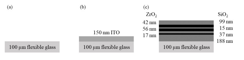
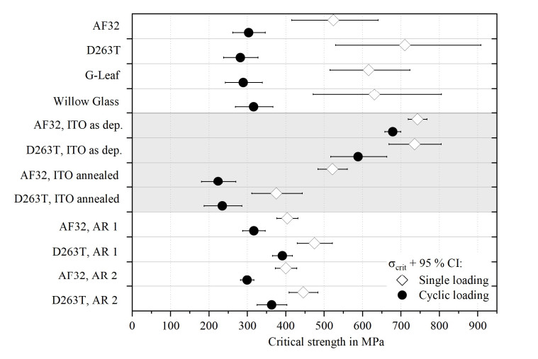
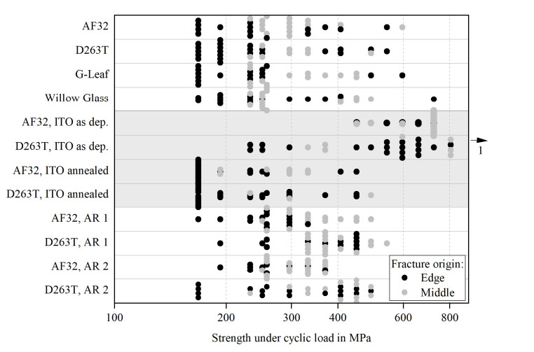
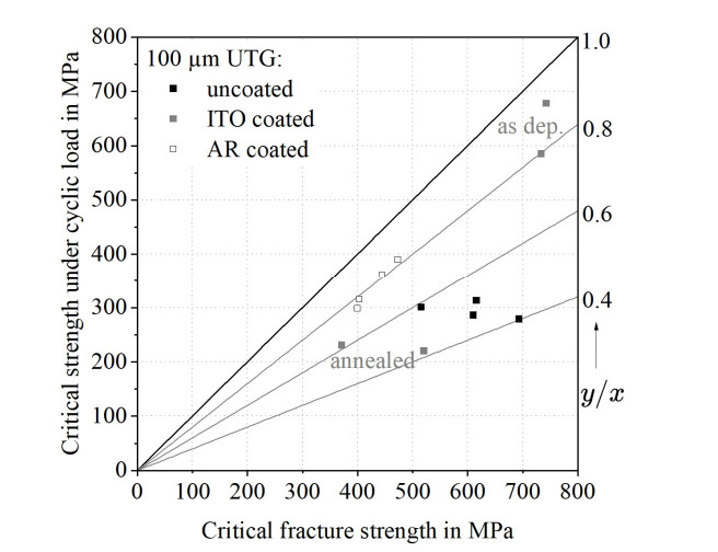
Ultra-thin flexible glass with thicknesses of 100 µm or below is a substrate in the fields of optics, electronics, and semiconductors. Its brittleness is challenging in production processes like physical vapor deposition processes, especially in roll-to-roll production. In many cases, multiple geometric deformations take place and each step, like coating or cutting, influences the glass strength. By now, the relation between the strength of ultra-thin glass under quasi-static conditions and its strength under cyclic load has not been studied. Moreover, the effect of coatings has not been investigated. Both aspects are crucial to design reliable production processes. Therefore, the strength of ultra-thin glass under cyclic load was studied for uncoated and coated substrates. Two coating types were investigated: a single indium tin oxide film and a seven-layer antireflective layer stack. The coatings significantly influence the strength of the underlying glass in both test modes. The barrier properties, thin film stress, and the morphology/crystalline structure are identified as the major characteristics influencing the strength.
Citation: Wiebke Langgemach, Andreas Baumann, Manuela Ehrhardt, Thomas Preußner, Edda Rädlein. The strength of uncoated and coated ultra-thin flexible glass under cyclic load[J]. AIMS Materials Science, 2024, 11(2): 343-368. doi: 10.3934/matersci.2024019
Ultra-thin flexible glass with thicknesses of 100 µm or below is a substrate in the fields of optics, electronics, and semiconductors. Its brittleness is challenging in production processes like physical vapor deposition processes, especially in roll-to-roll production. In many cases, multiple geometric deformations take place and each step, like coating or cutting, influences the glass strength. By now, the relation between the strength of ultra-thin glass under quasi-static conditions and its strength under cyclic load has not been studied. Moreover, the effect of coatings has not been investigated. Both aspects are crucial to design reliable production processes. Therefore, the strength of ultra-thin glass under cyclic load was studied for uncoated and coated substrates. Two coating types were investigated: a single indium tin oxide film and a seven-layer antireflective layer stack. The coatings significantly influence the strength of the underlying glass in both test modes. The barrier properties, thin film stress, and the morphology/crystalline structure are identified as the major characteristics influencing the strength.

| [1] | Garner SM, Li X, Huang MH (2017) Introduction to flexible glass substrates, In: Garner SM, Flexible Glass: Enabling Thin, Lightweight, and Flexible Electronics, Hoboken: John Wiley & Sons, 3–33. https://doi.org/10.1002/9781118946404 |
| [2] |
Weibull W (1951) A statistical distribution function of wide applicability. J Appl Mech 18: 293–297. https://doi.org/10.1115/1.4010337 doi: 10.1115/1.4010337

|
| [3] |
Ritter JE (1995) Predicting lifetimes of materials and material structures. Dent Mater 11: 142–146. https://doi.org/10.1016/0109-5641(95)80050-6 doi: 10.1016/0109-5641(95)80050-6
|
| [4] |
Griffith AA (1921) The phenomena of rupture and flow in solids. Philos T Roy Soc A 221: 163–198. https://doi.org/10.1098/rsta.1921.0006 doi: 10.1098/rsta.1921.0006
|
| [5] | Varner J (2003) Festigkeit und Bruchmechanik von Glas, In: Weißmann S, Varner J, Nattermann K, et al. Festigkeit von Glas—Grundlagen und Messverfahren, 2 Eds., Offenbach: Hüttentechnische Vereinigung der Deutschen Glasindustrie. |
| [6] | Lorenz G, Naumann F, Westphalen J, et al. (2016) Correlation of PVD deposition parameters with electrical and mechanical properties of coated thin-glass compounds. 6th Electronic System-Integration Technology Conference (13–15 September), Grenoble, IEEE, 1–6. https://doi.org/10.1109/ESTC.2016.7764740 |
| [7] | Glaesemann GS (2017) The mechanical reliability of thin, flexible glass, In: Garner SM, Flexible Glass: Enabling Thin, Lightweight, and Flexible Electronics, Hoboken: John Wiley & Sons, 35–62. https://doi.org/10.1002/9781118946404 |
| [8] | Jotz M (2022) Kantenfestigkeitsoptimierte (Weiter-) Entwicklung eines Verfahrens zum Trennen von ultradünnem Glas, Ilmenau: Universitätsverlag Ilmenau. https://doi.org/10.22032/dbt.53125 |
| [9] | Vineet K (2022) Transparent conductive films market. Available from: https://www.alliedmarketresearch.com/transparent-conductive-films-market. |
| [10] |
Glöß D, Frach P, Gottfried C, et al. (2008) Multifunctional high-reflective and antireflective layer systems with easy-to-clean properties. Thin Solid Films 516: 4487–4489. https://doi.org/10.1016/j.tsf.2007.05.097 doi: 10.1016/j.tsf.2007.05.097
|
| [11] |
Khan S, Wu H, Huai X, et al. (2018) Mechanically robust antireflective coatings. Nano Res 11: 1699–1713. https://doi.org/10.1007/s12274-017-1787-9 doi: 10.1007/s12274-017-1787-9
|
| [12] | German Institute for Standardization (2022) Load controlled fatigue testing—Execution and evaluation of cyclic tests at constant load amplitudes on metallic specimens and components. DIN 50100: 2022-12. |
| [13] | German Institute for Standardization (1990) Flexural fatigue testing of plastics using flat specimens. DIN 53442: 1990-09. |
| [14] | International Organization for Standardization (2003) Fibre-reinforced plastics—Determination of fatigue properties under cyclic loading conditions. ISO 13003: 2003. |
| [15] |
Evans AG (1974) Slow crack growth in brittle materials under dynamic loading conditions. Int J Fracture 10: 251–259. https://doi.org/10.1007/BF00113930 doi: 10.1007/BF00113930
|
| [16] |
Masuda M, Soma T, Matsui M (1990) Cyclic fatigue behavior of Si3N4 ceramics. J Eur Ceram Soc 6: 253–258. https://doi.org/10.1016/0955-2219(90)90052-H doi: 10.1016/0955-2219(90)90052-H
|
| [17] | Grenet L (1899) Recherches sur la résistance mécanique du verre: Mechanical strength of glass. Bulliten de la Societé d'Encouragement pour l'Industrie Nationale 5: 838–848. Available from: https://cnum.cnam.fr/pgi/redir.php?onglet = a & ident = BSPI. |
| [18] |
Gurney C, Pearson S (1948) Fatigue of mineral glass under static and cyclic loading. Philos T Roy Soc A 192: 537–544. https://doi.org/10.1098/rspa.1948.0025 doi: 10.1098/rspa.1948.0025
|
| [19] |
Lü BT (1997) Fatigue strength prediction of soda-lime glass. Theor Appl Fract Mec 27: 107–114. https://doi.org/10.1016/S0167-8442(97)00012-8 doi: 10.1016/S0167-8442(97)00012-8
|
| [20] |
Sglavo VM, Gadotti MT, Michelet T (1997) Cyclic loading behaviour of soda-lime silicate glass using indentation cracks. Fatigue Fract Eng M 20: 1225–1234. https://doi.org/10.1111/j.1460-2695.1997.tb00326.x doi: 10.1111/j.1460-2695.1997.tb00326.x
|
| [21] | Hilcken J (2015) Cyclic Fatigue of Annealed and Tempered Soda-Lime Glass, Berlin, Heidelberg: Springer. https://doi.org/10.1007/978-3-662-48353-4 |
| [22] |
Meyland MJ, Nielsen JH, Kocer C (2021) Tensile behaviour of soda-lime-silica glass and the significance of load duration—A literature review. J Build Eng 44: 102966. https://doi.org/10.1016/j.jobe.2021.102966 doi: 10.1016/j.jobe.2021.102966
|
| [23] |
Michalske TA, Freiman SW (1982) A molecular interpretation of stress corrosion in silica. Nature 295: 511–512. https://doi.org/10.1038/295511a0 doi: 10.1038/295511a0
|
| [24] |
Wiederhorn SM (1967) Influence of water vapor on crack propagation in soda-lime glass. J Am Ceram Soc 50: 407–414. https://doi.org/10.1111/j.1151-2916.1967.tb15145.x doi: 10.1111/j.1151-2916.1967.tb15145.x
|
| [25] |
Neugebauer J (2016) Determination of bending tensile strength of thin glass. Challenging Glass 5 Conference, 419–428. https://doi.org/10.7480/cgc.5.2267 doi: 10.7480/cgc.5.2267
|
| [26] | Heiß-Choquet M, Jotz M, Nattermann K, et al. (2014) Verfahren und Vorrichtung zur Bestimmung der Bruchfestigkeit der Ränder dünner Bahnen sprödbrüchigen Materials. German Patent DE 10 2014 110 855 B4. |
| [27] | Heiß-Choquet M, Jotz M, Nattermann K, et al. (2014)Verfahren und Vorrichtung zur Bestimmung der Kantenfestigkeit von scheibenförmigen Elementen aus sprödbrüchigem Material. German Patent DE 10 2014 110 856 B4. |
| [28] | Matthewson MJ, Kurkjian CR, Gulati ST (1986) Strength measurement of optical fibers by bending. J Am Ceram Soc 69: 815–821. https://doi.org/10.1111/j.1151-2916.1986.tb07366.x |
| [29] |
Gulati ST, Westbrook J, Carley S, et al. (2011) Two point bending of thin glass substrate. SID Int Symp Dig Tech Pap 42: 652–654. https://doi.org/10.1889/1.3621406 doi: 10.1889/1.3621406
|
| [30] |
Zaccaria M, Peters T, Ebert J, et al. (2022) The clamp bender: A new testing equipment for thin glass. Glass Struct Eng 7: 173–186. https://doi.org/10.1007/s40940-022-00188-8 doi: 10.1007/s40940-022-00188-8
|
| [31] | Langgemach W, Rädlein E (2024) A new method—Evaluation of the influence of coatings on the strength and fatigue strength of flexible glass. J Electron Mater (In press). |
| [32] | Schott AG (2022) AF32 eco: The alkali free answer to high technical demands, fact sheet. Available from: https://www.schott.com/de-de/products/af-32-eco-p1000308/downloads. |
| [33] | Schott AG (2023) D263T eco: The gold standard in imaging & sensing, fact sheet. Available from: https://www.schott.com/en-gb/products/d-263-P1000318/downloads. |
| [34] | Nippon Electric Glass Co., Ltd. (2024) Ultra-thin glass G-Leaf, fact sheet. Available from: https://www.neg.co.jp/en/assets/file/product/dp/en-g-leaf.pdf. |
| [35] | Corning Inc. (2019) The future is flexible: Corning willow glass, fact sheet. Available from: https://www.corning.com/media/worldwide/Innovation/documents/WillowGlass/Corning%20Willow%20Glass%20Fact%20Sheets_August2019.pdf. |
| [36] |
Juneja N, Tutsch L, Feldmann F, et al. (2019) Effect of hydrogen addition on bulk properties of sputtered indium tin oxide thin films. AIP Conf Proc 2147: 040008. https://doi.org/10.1063/1.5123835 doi: 10.1063/1.5123835
|
| [37] |
Stoney GG (1909) The tension of metallic films deposited by electrolysis. Proc R Soc Lond A 82: 172–175. https://doi.org/10.1098/rspa.1909.0021 doi: 10.1098/rspa.1909.0021
|
| [38] | Yuasa System Co., Ltd. (2023) Tension-free U-shape folding test. Available from: https://www.yuasa-system.jp/pdf/DLDMLH-FS_DLD-FS_en.pdf. |
| [39] |
Danzer R, Lube T, Supancic P, et al (2008) Fracture of ceramics. Adv Eng Mater 10: 275–298. https://doi.org/10.1002/adem.200700347 doi: 10.1002/adem.200700347
|
| [40] |
Mortazavian S, Fatemi A (2014) Notch effects on fatigue behavior of thermoplastics. Adv Mat Res 891–892: 1403–1409. https://doi.org/10.4028/www.scientific.net/AMR.891-892.1403 doi: 10.4028/www.scientific.net/AMR.891-892.1403
|
| [41] |
Prabhakaran R, Nair EMS, Sinha PK (1978) Notch sensitivity of polymers. J Appl Polym Sci 22: 3011–3020. https://doi.org/10.1002/app.1978.070221026 doi: 10.1002/app.1978.070221026
|
| [42] | Murakami Y (2002) Metal Fatigue: Effects of Small Defects and Nonmetallic Inclusions, 2 Eds., Cambridge, Massachusetts: Academic Press. https://doi.org/10.1016/C2016-0-05272-5 |
| [43] |
Neerinck DG, Vink TJ (1996) Depth profiling of thin ITO films by grazing incidence X-ray diffraction. Thin Solid Films 278: 12–17. https://doi.org/10.1016/0040-6090(95)08117-8 doi: 10.1016/0040-6090(95)08117-8
|
| [44] |
Mittelstedt C, Becker W (2004) Interlaminar stress concentrations in layered structures: Part Ⅰ—A selective literature survey on the free-edge effect since 1967. J Compos Mater 38: 1037–1062. https://doi.org/10.1177/0021998304040566 doi: 10.1177/0021998304040566
|
Figures(16) / Tables(6)

Wiebke Langgemach, Andreas Baumann, Manuela Ehrhardt, Thomas Preußner, Edda Rädlein. The strength of uncoated and coated ultra-thin flexible glass under cyclic load[J]. AIMS Materials Science, 2024, 11(2): 343-368. doi: 10.3934/matersci.2024019


 DownLoad: