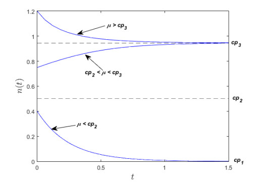
A nonautonomous logistic population model with a feature of an Allee threshold has been investigated in a periodically fluctuating environment. A slow periodicity of the harvesting effort was considered and may arise in response to relatively slow fluctuations of the environment. This assumption permits obtaining the analytical approximate solutions of such model using the perturbation approach based on the slow variation. Thus, the analytical expressions of the population evolution in the situation of subcritical and the supercritical harvesting were obtained and discussed in the framework of the Allee effect. Since the exact solution was not available due to the nonlinearity of the system, the numerical computation was considered to validate our analytical approximation. The comparison between the two methods showed a remarkable agreement as the time progressed, while such agreement fell off when the time was close to the initial density. Moreover, in the absence of the periodicity of the harvesting term, the expressions of the population evolution reduced to the exact solutions but in implicit forms. The finding results were appropriate for a wide range of parameter values, which lead to avoiding extensive recalculations while displaying the population behavior.
Citation: Fahad M. Alharbi. Harvesting a population model with Allee effect in a periodically varying environment[J]. AIMS Mathematics, 2024, 9(4): 8834-8847. doi: 10.3934/math.2024430
A nonautonomous logistic population model with a feature of an Allee threshold has been investigated in a periodically fluctuating environment. A slow periodicity of the harvesting effort was considered and may arise in response to relatively slow fluctuations of the environment. This assumption permits obtaining the analytical approximate solutions of such model using the perturbation approach based on the slow variation. Thus, the analytical expressions of the population evolution in the situation of subcritical and the supercritical harvesting were obtained and discussed in the framework of the Allee effect. Since the exact solution was not available due to the nonlinearity of the system, the numerical computation was considered to validate our analytical approximation. The comparison between the two methods showed a remarkable agreement as the time progressed, while such agreement fell off when the time was close to the initial density. Moreover, in the absence of the periodicity of the harvesting term, the expressions of the population evolution reduced to the exact solutions but in implicit forms. The finding results were appropriate for a wide range of parameter values, which lead to avoiding extensive recalculations while displaying the population behavior.

| [1] | R. B. Banks, Growth and diffusion phenomena: Mathematical frameworks and applications, Springer Science & Business Media, 14 (1993). |
| [2] | M. Braun, M. Golubitsky, Differential equations and their applications, Springer, 1 (1983). https://doi.org/10.1007/978-1-4684-0164-6-1 |
| [3] |
F. Courchamp, T. C. Brock, B. Grenfell, Inverse density dependence and the Allee effect, Trends Ecol. Evol., 14 (1999), 405–410. https://doi.org/10.1016/S0169-5347(99)01683-3 doi: 10.1016/S0169-5347(99)01683-3

|
| [4] |
P. A. Stephens, W. J. Sutherland, R. P. Freckleton, What is the Allee effect? Oikos, 1999,185–190. https://doi.org/10.2307/3547011 doi: 10.2307/3547011
|
| [5] | M. J. Panik, Stochastic differential equations: An introduction with applications in population dynamics modeling, John Wiley & Sons, 2017. https://doi.org/10.1002/9781119377399 |
| [6] |
M. Krstić, M. Jovanović, On stochastic population model with the Allee effect, Math. Comput. Model., 52 (2010), 370–379. https://doi.org/10.1016/j.mcm.2010.02.051 doi: 10.1016/j.mcm.2010.02.051
|
| [7] |
Q. Yang, D. Jiang, A note on asymptotic behaviors of stochastic population model with Allee effect, Appl. Math. Model., 35 (2011), 4611–4619. https://doi.org/10.1016/j.apm.2011.03.034 doi: 10.1016/j.apm.2011.03.034
|
| [8] |
J. R. Graef, S. Padhi, S. Pati, Periodic solutions of some models with strong Allee effects, Nonlinear Anal.-Real, 13 (2012), 569–581. https://doi.org/10.1016/j.nonrwa.2011.07.044 doi: 10.1016/j.nonrwa.2011.07.044
|
| [9] |
B. F. Brockett, M. Hassall, The existence of an Allee effect in populations of porcellio scaber (isopoda: Oniscidea), Eur. J. Soil Biol., 41 (2005), 123–127. https://doi.org/10.1016/j.ejsobi.2005.09.004 doi: 10.1016/j.ejsobi.2005.09.004
|
| [10] |
F. Courchamp, T. C. Brock, B. Grenfell, Inverse density dependence and the Allee effect, Trends Ecol. Evol., 14 (1999), 405–410. https://doi.org/10.1016/S0169-5347(99)01683-3 doi: 10.1016/S0169-5347(99)01683-3
|
| [11] |
F. M. Hilker, M. Langlais, S. V. Petrovskii, H. Malchow, A diffusive si model with Allee effect and application to FIV, Math. Biol., 206 (2007), 61–80. https://doi.org/10.1016/j.mbs.2005.10.003 doi: 10.1016/j.mbs.2005.10.003
|
| [12] |
A. Hurford, M. Hebblewhite, M. A. Lewis, A spatially explicit model for an Allee effect: Why wolves recolonize so slowly in greater yellowstone, Theor. Popul. Biol., 70 (2006), 244–254. https://doi.org/10.1016/j.tpb.2006.06.009 doi: 10.1016/j.tpb.2006.06.009
|
| [13] |
P. Amarasekare, Allee effects in metapopulation dynamics, Am. Nat., 152 (1998), 298–302. https://doi.org/10.1086/286169 doi: 10.1086/286169
|
| [14] |
M. A. Idlango, J. J. Shepherd, J. A. Gear, Multiscaling analysis of a slowly varying single species population model displaying an Allee effect, Math. Method. Appl. Sci., 37 (2014), 1561–1569. https://doi.org/10.1002/mma.2911 doi: 10.1002/mma.2911
|
| [15] |
A. Tesfay, D. Tesfay, J. Brannan, J. Duan, A logistic-harvest model with Allee effect under multiplicative noise, Stoch. Dynam., 21 (2021), 2150044. https://doi.org/10.1142/S0219493721500441 doi: 10.1142/S0219493721500441
|
| [16] |
F. B. Rizaner, S. P. Rogovchenko, Dynamics of a single species under periodic habitat fluctuations and Allee effect, Nonlinear Anal.-Real, 13 (2012), 141–157. https://doi.org/10.1016/j.nonrwa.2011.07.021 doi: 10.1016/j.nonrwa.2011.07.021
|
| [17] |
S. Rosenblat, Population models in a periodically fluctuating environment, J. Math. Biol., 9 (1980) 23–36. https://doi.org/10.1007/BF00276033 doi: 10.1007/BF00276033
|
| [18] |
T. Legović, G. Perić, Harvesting population in a periodic environment, Ecol. Model., 24 (1984), 221–229. https://doi.org/10.1016/0304-3800(84)90042-5 doi: 10.1016/0304-3800(84)90042-5
|
| [19] |
F. M. Alharbi, A slow single-species model with non-symmetric variation of the coefficients, Fractal Fract., 6 (2022), 72. https://doi.org/10.3390/fractalfract6020072 doi: 10.3390/fractalfract6020072
|
| [20] |
F. M. Alharbi, The general analytic expression of a harvested logistic model with slowly varying coefficients, Axioms, 11 (2022), 585. https://doi.org/10.3390/axioms11110585 doi: 10.3390/axioms11110585
|
| [21] |
A. K. Alsharidi, A. A. Khan, J. J. Shepherd, A. J. Stacey, Multiscaling analysis of a slowly varying anaerobic digestion model, Math. Method. Appl. Sci., 43 (2020), 5729–5743. https://doi.org/10.1002/mma.6315 doi: 10.1002/mma.6315
|
| [22] |
M. A. Idlango, J. J. Shepherd, J. A. Gear, Multiscaling analysis of a slowly varying single species population model displaying an Allee effect, Math. Method. Appl. Sci., 37 (2014), 1561–1569. https://doi.org/10.1002/mma.2911 doi: 10.1002/mma.2911
|
| [23] |
M. A. Idlango, J. J. Shepherd, J. A. Gear, Logistic growth with a slowly varying holling type Ⅱ harvesting term, Commun. Nonlinear Sci., 49 (2017), 81–92. https://doi.org/10.1016/j.cnsns.2017.02.005 doi: 10.1016/j.cnsns.2017.02.005
|
| [24] |
T. Cromer, Harvesting in a seasonal environment, Math. Comput. Model., 10 (1988), 445–450. https://doi.org/10.1016/0895-7177(88)90034-9 doi: 10.1016/0895-7177(88)90034-9
|
| [25] |
P. S. Meyer, J. H. Ausubel, Carrying capacity: A model with logistically varying limits, Technol. Forecast. Soc., 61 (1999), 209–214. https://doi.org/10.1016/S0040-1625(99)00022-0 doi: 10.1016/S0040-1625(99)00022-0
|
| [26] |
D. Ludwig, D. D. Jones, C. S. Holling, Qualitative analysis of insect outbreak systems: The spruce budworm and forest, J. Anim. Ecol., 47 (1978), 315–332. https://doi.org/10.2307/3939 doi: 10.2307/3939
|
| [27] |
J. J. Shepherd, L. Stojkov, The logistic population model with slowly varying carrying capacity, Anziam J., 47 (2005), C492–C506. https://doi.org/10.21914/anziamj.v47i0.1058 doi: 10.21914/anziamj.v47i0.1058
|
| [28] |
T. Grozdanovski, J. J. Shepherd, A. Stacey, Multi-scaling analysis of a logistic model with slowly varying coefficients, Appl. Math. Lett., 22 (2009), 1091–1095. https://doi.org/10.1016/j.aml.2008.10.002 doi: 10.1016/j.aml.2008.10.002
|
| [29] |
R. M. May, Thresholds and breakpoints in ecosystems with a multiplicity of stable states, Nature, 269 (1977), 471–477. https://doi.org/10.1038/269471a0 doi: 10.1038/269471a0
|


Figures(5) / Tables(1)

Fahad M. Alharbi. Harvesting a population model with Allee effect in a periodically varying environment[J]. AIMS Mathematics, 2024, 9(4): 8834-8847. doi: 10.3934/math.2024430


 DownLoad: