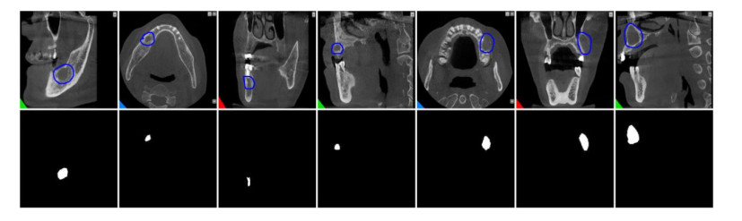
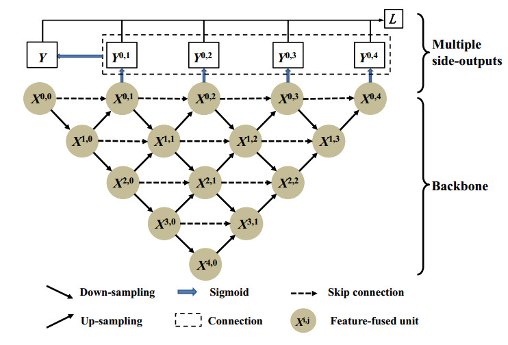
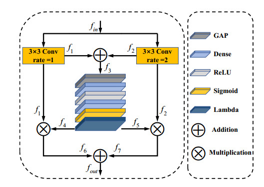
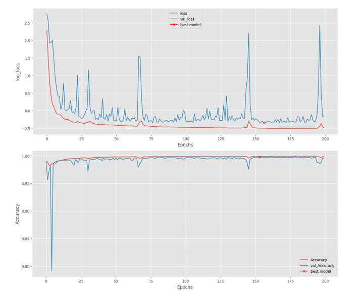
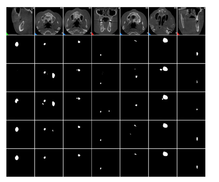
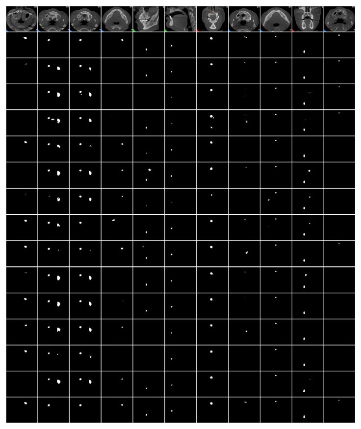
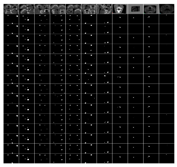
Jaw cysts are mainly caused by abnormal tooth development, chronic oral inflammation, or jaw damage, which may lead to facial swelling, deformity, tooth loss, and other symptoms. Due to the diversity and complexity of cyst images, deep-learning algorithms still face many difficulties and challenges. In response to these problems, we present a horizontal-vertical interaction and multiple side-outputs network for cyst segmentation in jaw images. First, the horizontal-vertical interaction mechanism facilitates complex communication paths in the vertical and horizontal dimensions, and it has the ability to capture a wide range of context dependencies. Second, the feature-fused unit is introduced to adjust the network's receptive field, which enhances the ability of acquiring multi-scale context information. Third, the multiple side-outputs strategy intelligently combines feature maps to generate more accurate and detailed change maps. Finally, experiments were carried out on the self-established jaw cyst dataset and compared with different specialist physicians to evaluate its clinical usability. The research results indicate that the Matthews correlation coefficient (Mcc), Dice, and Jaccard of HIMS-Net were 93.61, 93.66 and 88.10% respectively, which may contribute to rapid and accurate diagnosis in clinical practice.
Citation: Xiaoliang Jiang, Huixia Zheng, Zhenfei Yuan, Kun Lan, Yaoyang Wu. HIMS-Net: Horizontal-vertical interaction and multiple side-outputs network for cyst segmentation in jaw images[J]. Mathematical Biosciences and Engineering, 2024, 21(3): 4036-4055. doi: 10.3934/mbe.2024178
Jaw cysts are mainly caused by abnormal tooth development, chronic oral inflammation, or jaw damage, which may lead to facial swelling, deformity, tooth loss, and other symptoms. Due to the diversity and complexity of cyst images, deep-learning algorithms still face many difficulties and challenges. In response to these problems, we present a horizontal-vertical interaction and multiple side-outputs network for cyst segmentation in jaw images. First, the horizontal-vertical interaction mechanism facilitates complex communication paths in the vertical and horizontal dimensions, and it has the ability to capture a wide range of context dependencies. Second, the feature-fused unit is introduced to adjust the network's receptive field, which enhances the ability of acquiring multi-scale context information. Third, the multiple side-outputs strategy intelligently combines feature maps to generate more accurate and detailed change maps. Finally, experiments were carried out on the self-established jaw cyst dataset and compared with different specialist physicians to evaluate its clinical usability. The research results indicate that the Matthews correlation coefficient (Mcc), Dice, and Jaccard of HIMS-Net were 93.61, 93.66 and 88.10% respectively, which may contribute to rapid and accurate diagnosis in clinical practice.

| [1] |
P. Wang, J. Z. Peng, M. Pedersoli, Y. F. Zhou, C. M. Zhang, C. Desrosiers, CAT: Constrained adversarial training for anatomically-plausible semi-supervised segmentation, IEEE Trans. Med. Imaging, 42 (2023), 2146–2161. https://doi.org/10.1109/TMI.2023.3243069 doi: 10.1109/TMI.2023.3243069

|
| [2] |
L. Zhang, K. J. Zhang, H. W. Pan, SUNet plus plus: A deep network with channel attention for small-scale object segmentation on 3D medical images, Tsinghua Sci. Technol., 28 (2023), 628–638. https://doi.org/10.26599/TST.2022.9010023 doi: 10.26599/TST.2022.9010023
|
| [3] |
D. D. Meng, S. Li, B. Sheng, H. Wu, S. Q. Tian, W. J. Ma, et al., 3D reconstruction-oriented fully automatic multi-modal tumor segmentation by dual attention-guided VNet, Visual Comput., 39 (2023), 3183–3196. https://doi.org/10.1007/s00371-023-02965-0 doi: 10.1007/s00371-023-02965-0
|
| [4] |
Y. Feng, Y. H. Wang, H. H. Li, M. J. Qu, J. Z. Yang, Learning what and where to segment: A new perspective on medical image few-shot segmentation, Med. Image Anal., 87 (2023), 102834. https://doi.org/10.1016/j.media.2023.102834 doi: 10.1016/j.media.2023.102834
|
| [5] |
Y. X. Ma, S. Wang, Y. Hua, R. H. Ma, T. Song, Z. G. Xue, et al. Perceptual data augmentation for biomedical coronary vessel segmentation, IEEE/ACM Trans. Comput. Biol. Bioinf., 20 (2023), 2494–2505. https://doi.org/10.1109/TCBB.2022.3188148 doi: 10.1109/TCBB.2022.3188148
|
| [6] | O. Ronneberger, P. Fischer, T. Brox, U-net: Convolutional networks for biomedical image segmentation, in International Conference on Medical Image Computing and Computer-assisted Intervention, Munich, Germany, (2015), 234–241. https://doi.org/10.1007/978-3-319-24574-4_28 |
| [7] |
A. Sharma, P. K. Mishra, DRI-UNet: dense residual-inception UNet for nuclei identification in microscopy cell images, Neural Comput. Appl., 35 (2023), 19187–19220. https://doi.org/10.1007/s00521-023-08729-0 doi: 10.1007/s00521-023-08729-0
|
| [8] |
B. Sarica, D. Z. Seker, B. Bayram, A dense residual U-net for multiple sclerosis lesions segmentation from multi-sequence 3D MR images, Int. J. Med. Inf., 170 (2023), 104965. https://doi.org/10.1016/j.ijmedinf.2022.104965 doi: 10.1016/j.ijmedinf.2022.104965
|
| [9] |
Q. Xu, Z. Ma, H. E. Na, W. Duan, DCSAU-Net: A deeper and more compact split-attention U-Net for medical image segmentation, Comput. Biol. Med., 154 (2023), 106626. https://doi.org/10.1016/j.compbiomed.2023.106626 doi: 10.1016/j.compbiomed.2023.106626
|
| [10] |
H. Wang, G. Xu, X. Pan, Z. Liu, N. Tang, R. Lan, et al., Attention-inception-based U-Net for retinal vessel segmentation with advanced residual, Comput. Electr. Eng., 98 (2022), 107670. https://doi.org/10.1016/j.compeleceng.2021.107670 doi: 10.1016/j.compeleceng.2021.107670
|
| [11] |
J. Zhang, Y. Zhang, Y. Jin, J. Xu, X. Xu, MDU-Net: multi-scale densely connected U-Net for biomedical image segmentation, Health Inf. Sci. Syst., 11 (2023), 13. https://doi.org/10.1007/s13755-022-00204-9 doi: 10.1007/s13755-022-00204-9
|
| [12] |
S. Banerjee, J. Lyu, Z. Huang, F. H. Leung, T. Lee, D. Yang, et al., Ultrasound spine image segmentation using multi-scale feature fusion skip-inception U-Net (SIU-Net), Biocybern. Biomed. Eng., 42 (2022), 341–361. https://doi.org/10.1016/j.bbe.2022.02.011 doi: 10.1016/j.bbe.2022.02.011
|
| [13] |
S. Wang, V. K. Singh, E. Cheah, X. Wang, Q. Li, S. H. Chou, et al., Stacked dilated convolutions and asymmetric architecture for U-Net-based medical image segmentation, Comput. Biol. Med., 148 (2022), 105891. https://doi.org/10.1016/j.compbiomed.2022.105891 doi: 10.1016/j.compbiomed.2022.105891
|
| [14] |
J. Mutaguchi, K. I. Morooka, S. Kobayashi, A. Umehara, S. Miyauchi, F. Kinoshita, et al., Artificial intelligence for segmentation of bladder tumor cystoscopic images performed by U-Net with dilated convolution, J. Endourol., 36 (2022), 827–834. https://doi.org/10.1089/end.2021.0483 doi: 10.1089/end.2021.0483
|
| [15] |
J. Vidal, J. C. Vilanova, R. Martí, A U-Net ensemble for breast lesion segmentation in DCE MRI, Comput. Biol. Med., 140 (2022), 105093. https://doi.org/10.1016/j.compbiomed.2021.105093 doi: 10.1016/j.compbiomed.2021.105093
|
| [16] |
K. Sun, Y. Xin, Y. Ma, M. Lou, Y. Qi, J. Zhu, ASU-Net: U-shape adaptive scale network for mass segmentation in mammograms, J. Intell. Fuzzy Syst., 42 (2022), 4205–4220. https://doi.org/10.3233/JIFS-210393 doi: 10.3233/JIFS-210393
|
| [17] |
F. Abdolali, R. A. Zoroofi, Y. Otake, Y. Sato, Automatic segmentation of maxillofacial cysts in cone beam CT images, Comput. Biol. Med., 72 (2016), 108–119. https://doi.org/10.1016/j.compbiomed.2016.03.014 doi: 10.1016/j.compbiomed.2016.03.014
|
| [18] |
M. K. Alsmadi, A hybrid Fuzzy C-means and Neutrosophic for jaw lesions segmentation, Ain Shams Eng. J., 9 (2018), 697–706. https://doi.org/10.1016/j.asej.2016.03.016 doi: 10.1016/j.asej.2016.03.016
|
| [19] | J. Hu, Z. Feng, Y. Mao, J. Lei, D. Yu, M. Song, A location constrained dual-branch network for reliable diagnosis of jaw tumors and cysts, in International Conference of Medical Image Computing and Computer Assisted Intervention, Strasbourg, France, (2021), 723–732. https://doi.org/10.1007/978-3-030-87234-2_68 |
| [20] |
S. Sivasundaram, C. Pandian, Performance analysis of classification and segmentation of cysts in panoramic dental images using convolutional neural network architecture, Int. J. Imaging Syst. Technol., 31 (2021), 2214–2225. https://doi.org/10.1002/ima.22625 doi: 10.1002/ima.22625
|
| [21] |
D. K. Veena, A. Jatti, M. J. Vidya, R. Joshi, S. Gade, A novel approach towards automatic contour identification of jaw cysts from digital panoramic radiographs to improvise the treatment planning, Int. J. Biol. Biomed. Eng., 16 (2022), 1–8. https://doi.org/10.46300/91011.2022.16.1 doi: 10.46300/91011.2022.16.1
|
| [22] | Z. W. Zhou, M. M. R. Siddiquee, N. Tajbakhsh, J. M. Liang, UNet++: A nested U-Net architecture for medical image segmentation, in Deep Learning in Medical Image Analysis and Multimodal Learning for Clinical Decision Support, Granada, Spain, (2018), 3–11. https://doi.org/10.1007/978-3-030-00889-5_1 |
| [23] |
Z. Zhou, M. M. R. Siddiquee, N. Tajbakhsh, J. Liang, UNet++: Redesigning Skip Connections to Exploit Multiscale Features in Image Segmentation, IEEE Trans. Med. Imaging, 39 (2020), 1856–1867. https://doi.org/10.1109/TMI.2019.2959609 doi: 10.1109/TMI.2019.2959609
|
| [24] | K. Sun, B. Xiao, D. Liu, J. Wang, Deep high-resolution representation learning for human pose estimation, in IEEE International Conference on Computer Vision & Pattern Recognition, Long Beach, CA, USA, (2019), 5686–5696. https://doi.org/10.1109/CVPR.2019.00584 |
| [25] |
M. Zhao, Y. Wei, Y. Lu, K. K. L. Wong, A novel U-Net approach to segment the cardiac chamber in magnetic resonance images with ghost artifacts, Comput. Methods Programs Biomed., 196 (2020), 105623. https://doi.org/10.1016/j.cmpb.2020.105623 doi: 10.1016/j.cmpb.2020.105623
|
| [26] |
A. S. Mahmoud, S. A. Mohamed, R. A. El-Khoriby, H. M. AbdelSalam, I. A. El-Khodary, Oil spill identification based on dual attention UNet model using synthetic aperture radar images, J. Indian Soc. Remote Sens., 51 (2023), 121–133. https://doi.org/10.1007/s12524-022-01624-6 doi: 10.1007/s12524-022-01624-6
|
| [27] |
X. Xie, X. Pan, W. Zhang, J. An, A context hierarchical integrated network for medical image segmentation, Comput. Electr. Eng., 101 (2022), 108029. https://doi.org/10.1016/j.compeleceng.2022.108029 doi: 10.1016/j.compeleceng.2022.108029
|
| [28] |
L. Zhu, L. Zhang, W. Hu, H. Chen, H. Li, S. Wei, et al., A multi-task two-path deep learning system for predicting the invasiveness of craniopharyngioma, Comput. Meth. Prog. Bio., 216 (2022), 106651. https://doi.org/10.1016/j.cmpb.2022.106651 doi: 10.1016/j.cmpb.2022.106651
|
| [29] |
L. Zhang, Y. Liao, G. Wang, J. Chen, H. Wang, A multi-scale contextual information enhancement network for crack segmentation, Appl. Sci., 12 (2022), 11135. https://doi.org/10.3390/app122111135 doi: 10.3390/app122111135
|
| [30] |
M. Jiang, X. Zhang, Y. Sun, W. Feng, Q. Gan, Y. Ruan, AFSNet: Attention-guided full-scale feature aggregation network for highresolution remote sensing image change detection, GISci. Remote Sens., 59 (2022), 1882–1900. https://doi.org/10.1080/15481603.2022.2142626 doi: 10.1080/15481603.2022.2142626
|
| [31] |
C. Xu, Y. Qi, Y. Wang, M. Lou, J. Pi, Y. Ma, ARF-Net: An adaptive receptive field network for breast masssegmentation in whole mammograms and ultrasound images, Biomed. Signal Process. Control, 71 (2022), 103178. https://doi.org/10.1016/j.bspc.2021.103178 doi: 10.1016/j.bspc.2021.103178
|
| [32] |
D. Maji, P. Sigedar, M. Singh, Attention Res-UNet with guided decoder for semantic segmentation of brain tumors, Biomed. Signal Process. Control, 71 (2022), 103077. https://doi.org/10.1016/j.bspc.2021.103077 doi: 10.1016/j.bspc.2021.103077
|
| [33] | H. Huang, L. Lin, R. Tong, H. Hu, J. Wu, UNet 3+: A full-scale connected UNet for medical image segmentation, in IEEE International Conference on Acoustics, Speech and Signal Processing, Barcelona, Spain, (2020), 1055–1059. https://doi.org/10.1109/ICASSP40776.2020.9053405 |
| [34] |
K. Wang, S. Liang, S. Zhong, Q. Feng, Y. Zhang, Breast ultrasound image segmentation: A coarse-to-fine fusion convolutional neural network, Med. Phys., 48 (2021), 4262–4278. https://doi.org/10.1002/mp.15006 doi: 10.1002/mp.15006
|
| [35] |
J. Wang, P. Lv, H. Wang, C. Shi, SAR-U-Net: Squeeze-and-excitation block and atrous spatial pyramid pooling based residual U-Net for automatic liver ct segmentation, Comput. Methods Programs Biomed., 208 (2021), 106268. https://doi.org/10.1016/j.cmpb.2021.106268 doi: 10.1016/j.cmpb.2021.106268
|
| [36] |
G. Xiao, B. Zhu, Y. Zhang, H. Gao, FCSNet: A quantitative explanation method for surface scratch defects during belt grinding based on deep learning, Comput. Ind., 144 (2023), 103793. https://doi.org/10.1016/j.compind.2022.103793 doi: 10.1016/j.compind.2022.103793
|
| [37] |
A. Iqbal, M. Sharif, M. A. Khan, W. Nisar, M. Alhaisoni, FF-UNet: A u-shaped deep convolutional neural network for multimodal biomedical image segmentation, Cognit. Comput., 14 (2022), 1287–1302. https://doi.org/10.1007/s12559-022-10038-y doi: 10.1007/s12559-022-10038-y
|
| [38] |
F. Xie, Z. Huang, Z. Shi, T. Wang, G. Song, B. Wang, et al., DUDA-Net: A double u-shaped dilated attention network for automatic infection area segmentation in COVID-19 lung CT images, Int. J. Comput. Assisted Radiol. Surg., 16 (2021), 1425–1434. https://doi.org/10.1007/s11548-021-02418-w doi: 10.1007/s11548-021-02418-w
|
| [39] | R. Azad, M. Asadi-Aghbolaghi, M. Fathy, S. Escalera, Bi-directional ConvLSTM U-Net with densley connected convolutions, in Proceedings of the IEEE/CVF International Conference on Computer Vision workshops, Seoul, Korea, (2019), 406–415. https://doi.org/10.1109/ICCVW.2019.00052 |
| [40] |
D. Peng, Y. Zhang, H. Guan, End-to-end change detection for high resolution satellite images using improved UNet++, Remote Sens., 11 (2019), 1382. https://doi.org/10.3390/rs11111382 doi: 10.3390/rs11111382
|
| [41] |
H. Wu, Z. Zhao, Z. Wang, META-Unet: Multi-scale efficient transformer attention Unet for fast and high-accuracy polyp segmentation, IEEE Trans. Autom. Sci. Eng., (2023), 1–12. https://doi.org/10.1109/TASE.2023.3292373 doi: 10.1109/TASE.2023.3292373
|
| [42] |
R. Su, D. Zhang, J. Liu, C. Cheng, MSU-Net: Multi-scale U-Net for 2D medical image segmentation, Front. Genet., 12 (2021), 639930. https://doi.org/10.3389/fgene.2021.639930 doi: 10.3389/fgene.2021.639930
|
| [43] |
Z. Gu, J. Cheng, H. Fu, K. Zhou, H. Hao, Y. Zhao, et al., CE-Net: Context encoder network for 2d medical image segmentation, IEEE Trans. Med. Imaging, 38 (2019), 2281–2292. https://doi.org/10.1109/TMI.2019.2903562 doi: 10.1109/TMI.2019.2903562
|
| [44] |
M. M. Ji, Z. B. Wu, Automatic detection and severity analysis of grape black measles disease based on deep learning and fuzzy logic, Comput. Electron. Agric., 193 (2022), 106718. https://doi.org/10.1016/j.compag.2022.106718 doi: 10.1016/j.compag.2022.106718
|
| [45] |
M. Jiang, F. Zhai, J. Kong, A novel deep learning model DDU-net using edge features to enhance brain tumor segmentation on MR images, Artif. Intell. Med., 121 (2021), 102180. https://doi.org/10.1016/j.artmed.2021.102180 doi: 10.1016/j.artmed.2021.102180
|
| [46] |
Y. Y. Yang, C. Feng, R. F. Wang, Automatic segmentation model combining U-Net and level set method for medical images, Expert Syst. Appl., 153 (2020), 113419. https://doi.org/10.1016/j.eswa.2020.113419 doi: 10.1016/j.eswa.2020.113419
|
| [47] |
C. Zhao, R. J. Shuai, L. Ma, W. J. Liu, M. L. Wu, Segmentation of dermoscopy images based on deformable 3D convolution and ResU-NeXt++, Med. Biol. Eng. Comput., 59 (2021), 1815–1832. https://doi.org/10.1007/s11517-021-02397-9 doi: 10.1007/s11517-021-02397-9
|
Figures(7) / Tables(6)

Xiaoliang Jiang, Huixia Zheng, Zhenfei Yuan, Kun Lan, Yaoyang Wu. HIMS-Net: Horizontal-vertical interaction and multiple side-outputs network for cyst segmentation in jaw images[J]. Mathematical Biosciences and Engineering, 2024, 21(3): 4036-4055. doi: 10.3934/mbe.2024178


 DownLoad: