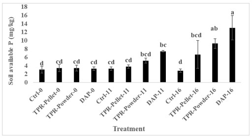
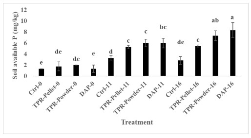
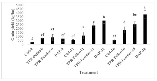
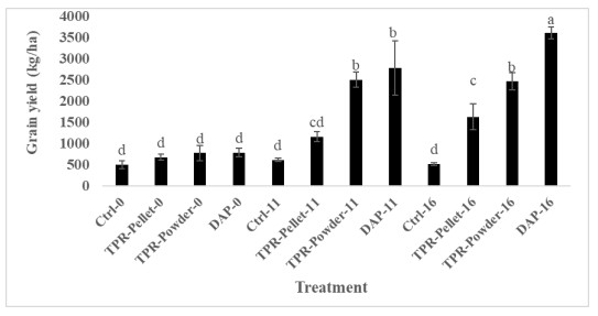
Crop yield in sub-Saharan Africa is often limited by low phosphorus fertility. Farmers in the region can apply phosphate rock, which should increase the plant-available phosphorus level, but this may be prone to sorption in acid soils of the Sahel. The objective of this study was to determine phosphorus (P) sorption characteristics of four representative soil series in Sahelian Mali namely, Longorola (Gleysol), Danga (Fluvisol), Niessoumana (Arenosol) and Konobougou (Acrisol) under Tilemsi Phosphate Rock (TPR) treatment. Data for phosphorus sorption was obtained by equilibrating 5 g of soils for 7 days at room temperature in 50 ml of 0.01M CaCl2 containing six (6) rates of phosphate as TPR (0, 10, 20, 40, 80,160 mg/L). The linear form of the Langmuir equation was used to calculate sorption parameters of the soils. The Gleysol with the greatest clay content had the highest phosphorus sorption maximum which was over three times greater than that of the Acrisol with the least clay content. The sorption maxima in the range of 59–200 mg/kg were well estimated with Langmuir sorption isotherm (R2 ≥ 0.78). Soil organic matter and clay contents influenced phosphorus sorption from the TPR. The degree of phosphorus saturation ranged from 2.39 to 6.47 %, being greater in the Arenosol. In a two-season field experiment on the Haplic Acrisol, we tested on maize, the TPR in two forms (powder and pellet) in addition to water-soluble diammonium phosphate at different rates (0, 11 and 16 kg P /ha). The water-soluble DAP and TPR (powder) had similar effects (p < 0.05) on soil P availability but with DAP producing greater grain yields. This shows that application of TPR in powder form can improve phosphorus availability as water-soluble DAP with positive impact on grain yield. The study provides useful information on P sorption characteristics of TPR amendment in the Sahel.
Citation: Aliou Badara Kouyate, Vincent Logah, Robert Clement Abaidoo, Francis Marthy Tetteh, Mensah Bonsu, Sidiki Gabriel Dembélé. Phosphorus sorption characteristics in the Sahel: Estimates from soils in Mali[J]. AIMS Agriculture and Food, 2023, 8(4): 995-1009. doi: 10.3934/agrfood.2023053
Crop yield in sub-Saharan Africa is often limited by low phosphorus fertility. Farmers in the region can apply phosphate rock, which should increase the plant-available phosphorus level, but this may be prone to sorption in acid soils of the Sahel. The objective of this study was to determine phosphorus (P) sorption characteristics of four representative soil series in Sahelian Mali namely, Longorola (Gleysol), Danga (Fluvisol), Niessoumana (Arenosol) and Konobougou (Acrisol) under Tilemsi Phosphate Rock (TPR) treatment. Data for phosphorus sorption was obtained by equilibrating 5 g of soils for 7 days at room temperature in 50 ml of 0.01M CaCl2 containing six (6) rates of phosphate as TPR (0, 10, 20, 40, 80,160 mg/L). The linear form of the Langmuir equation was used to calculate sorption parameters of the soils. The Gleysol with the greatest clay content had the highest phosphorus sorption maximum which was over three times greater than that of the Acrisol with the least clay content. The sorption maxima in the range of 59–200 mg/kg were well estimated with Langmuir sorption isotherm (R2 ≥ 0.78). Soil organic matter and clay contents influenced phosphorus sorption from the TPR. The degree of phosphorus saturation ranged from 2.39 to 6.47 %, being greater in the Arenosol. In a two-season field experiment on the Haplic Acrisol, we tested on maize, the TPR in two forms (powder and pellet) in addition to water-soluble diammonium phosphate at different rates (0, 11 and 16 kg P /ha). The water-soluble DAP and TPR (powder) had similar effects (p < 0.05) on soil P availability but with DAP producing greater grain yields. This shows that application of TPR in powder form can improve phosphorus availability as water-soluble DAP with positive impact on grain yield. The study provides useful information on P sorption characteristics of TPR amendment in the Sahel.

| [1] | Bationo A, Rhodes E, Smaling EMA, et al. (1996) Technologies for restoring soil fertility. In: Restoring and maintaining the productivity of West African soils: Key to sustainable development, 61–72. Available from: https://pdf.usaid.gov/pdf_docs/PNABY620.pdf. |
| [2] |
Boureima S, Mahaman IL (2020) Effets de la déficience en phosphore du sol sur la croissance et le développement du Sésame (Sesanum indicum L.). Int J Biol Chem Sci 14: 1014–1024. https://doi.org/10.4314/ijbcs.v14i3.28 doi: 10.4314/ijbcs.v14i3.28

|
| [3] | Pierzynski GM, McDowell RW, Sim TJ (2005) Chemistry, cycling, and potential movement of inorganic phosphorus in soils. In: Phosphorus: Agriculture and the environment. American Society of Agronomy, Inc., Crop Science Society. https://doi.org/10.2134/agronmonogr46.c3 |
| [4] | Lindsay WL, Vlek PLG, Chien SH (1989) Phosphate minerals. In: Dixon JB, Weed SB (Eds) Minerals in soil environments, Soil Science Society of America, Inc. https://doi.org/10.2136/sssabookser1.2ed.c22 |
| [5] |
Devau N, Le Cadre, E, Hinsinger P, et al. (2010) A mechanistic model for understanding root-induced chemical changes controlling phosphorus availability. Ann Bot 105: 1183–1197. https://doi.org/10.1093/aob/mcq098 doi: 10.1093/aob/mcq098
|
| [6] |
Debicka M, Kocowicz, A, Weber J, et al. (2016) Organic matter effects on phosphorus sorption in sandy soils. Arch Agron Soil Sci 62: 840–855. https://doi.org/10.1080/03650340.2015.1083981 doi: 10.1080/03650340.2015.1083981
|
| [7] |
Ohno T, Griffin TS, Liebman M, et al. (2005) Chemical characterization of soil phosphorus and organic matter in different cropping systems in Maine, U.S.A. Agr Ecosyst Environ 105: 625–634. https://doi.org/10.1016/j.agee.2004.08.001 doi: 10.1016/j.agee.2004.08.001
|
| [8] |
Babana AH, Antoun H (2006) Effect of Tilemsi phosphate rock-solubilizing microorganisms on phosphorus uptake and yield of field-grown wheat (Triticum aestivum L.) in Mali. Plant Soil 287: 51–58. https://doi.org/10.1007/s11104-006-9060-0 doi: 10.1007/s11104-006-9060-0
|
| [9] |
Bationo A, Ayuk E, Ballo D, et al. (1997) Agronomic and economic evaluation of Tilemsi phosphate rock in different agroecological zones of Mali. Nutr Cycl Agroecosys 48: 179–189. https://doi.org/10.1023/A:1009784812549 doi: 10.1023/A:1009784812549
|
| [10] | FAO (Food and Agriculture Organization) (1990) Soil Map of the World—Revised Legend. 4th Draft, Rome. |
| [11] | Keita B (2000) Les sols dominants du Mali. In: Quatorzième Réunion du Sous-Comité ouest et centre africain de corrélation des sols pour la mise en valeur des terres, Available from: https://www.fao.org/3/y3948f/y3948f00.htm#toc. |
| [12] |
Anderson JM, Ingram JSI (1990) Tropical soil biology and fertility: A handbook of methods. J Ecol 78: 547–548. https://doi.org/10.2307/2261129 doi: 10.2307/2261129
|
| [13] |
Nelson DW, Sommers LE (1982) Total nitrogen analysis for soil and plant tissues. J Assoc Off Anal Chem 63: 770–778. https://doi.org/10.1093/jaoac/63.4.770 doi: 10.1093/jaoac/63.4.770
|
| [14] | Rhoades JD (1982) Cation exchange capacity. In: Methods of soil analysis. Part 2. 2nd ed. Agronomy. Monograph. 9. ASA and SSSA, Madison, WI. |
| [15] |
Hue NV, Fox RL (2010) Predicting plant phosphorus requirements for Hawaii soils using a combination of phosphorus sorption isotherms and chemical extraction methods. Commun Soil Sci Plant Anal 4: 133–143. https://doi.org/10.1080/00103620903426949 doi: 10.1080/00103620903426949
|
| [16] |
Guo X, Wang J (2019) Comparison of linearization methods for modeling the Langmuir adsorption isotherm. J Mol Liq 296: 11850. https://doi.org/10.1016/j.molliq.2019.111850 doi: 10.1016/j.molliq.2019.111850
|
| [17] |
Paultley MC, Sims JT (2000) Relationships between soil phosphorus, soluble phosphorus saturation in Delaware soils. Soil Sci Soc Am J 64: 765–773. https://doi.org/10.2136/sssaj2000.642765x doi: 10.2136/sssaj2000.642765x
|
| [18] |
Kablan R, Yost RS, Brannan K, et al. (2008) Aménagement en courbes de niveau "Increasing rainfall capture, storage, and drainage in soils of Mali. Ari Land Res Manag 22: 62–80. https://doi.org/10.1080/15324980701784191 doi: 10.1080/15324980701784191
|
| [19] |
Tamungang NEB, Mvondo-Ze AD, Ghogomu, JN, et al. (2016). Evaluation of phosphorus sorption characteristics of soils from the Bambouto sequence (West Cameroon). Int J Biol Chem Sci 10: 860–874. https://doi.org/10.4314/ijbcs.v10i2.33 doi: 10.4314/ijbcs.v10i2.33
|
| [20] |
Hanyabui E, Apori SO, Frimpong KA, et al. (2020) Phosphorus sorption in tropical soils. AIMS Agric Food 5: 599–616. https://doi.org/10.3934/agrfood.2020.4.599 doi: 10.3934/agrfood.2020.4.599
|
| [21] |
Wang X, Yost RS, Linquist BA (2001) Soil aggregate size affects phosphorus desorption from highly weathered soils and plant growth. Soil Sci Soc Am J 65: 139–146. https://doi.org/10.2136/sssaj2001.651139x doi: 10.2136/sssaj2001.651139x
|
| [22] | Pissarides AS (1996) Phosphorus adsorption by selected clay minerals. Ph D Thesis, University of Saskatchewan. Available from: http://hdl.handle.net/10388/etd-10042010-081741. |
| [23] |
Borggard OK, Jorgensen SS, Moberg JP, et al. (1990) Influence of organic matter on phosphate adsorption by aluminium and iron oxides in sandy soils. J Soil Sci 41: 443–449. https://doi.org/10.1111/j.1365-2389.1990.tb00078.x doi: 10.1111/j.1365-2389.1990.tb00078.x
|
| [24] |
Yang X. Chen X, Yang Y (2019) Effect of organic matter on phosphorus adsorption and desorption in a black soil from Northeast China. Soil Till Res 187: 85–91. https://doi.org/10.1016/j.still.2018.11.016 doi: 10.1016/j.still.2018.11.016
|
| [25] |
Hiradate S, Uchida N (2004) Effects of soil organic matter on pH-dependent phosphate sorption by soils. Soil Sci Plant Nutr 50: 665–675. https://doi.org/10.1080/00380768.2004.10408523 doi: 10.1080/00380768.2004.10408523
|
| [26] |
Wang L, Liang T (2014) Effects of exogenous rare earth elements on phosphorus adsorption and desorption in different types of soils. Chemosphere 103: 148–155. https://doi.org/10.1016/j.chemosphere.2013.11.050 doi: 10.1016/j.chemosphere.2013.11.050
|
| [27] |
Bortoluzzi EC, Pérez CAS, Ardisson JD, et al. (2015) Occurrence of iron and aluminum sesquioxides and their implications for the P sorption in subtropical soils. Appl Clay Sci 104: 196–204. https://doi.org/10.1016/j.clay.2014.11.032 doi: 10.1016/j.clay.2014.11.032
|
| [28] |
Hunt JF, Ohno T, He Z (2007) Inhibition of phosphorus sorption to goethite, gibbsite, and kaolin by fresh and decomposed organic matter. Biol Fertil Soil 44: 277–288. https://doi.org/10.1007/s00374-007-0202-1 doi: 10.1007/s00374-007-0202-1
|
| [29] | Sample EC, Soper RJ, Racz GJ (1980) Reactions of phosphate fertilizers in soils. In: The role of phosphorus in agriculture 55: 90–95. https://doi.org/10.2134/1980.roleofphosphorus.c12 |
| [30] |
Tening AS, Foba-Tendo JN, Yakum-Ntaw SY, et al. (2013). Phosphorus fixing capacity of a volcanic soil on the slope of mount Cameroon. Agric Biol J N Am 4: 166–174. https://doi.org/10.5251/abjna.2013.4.3.166.174 doi: 10.5251/abjna.2013.4.3.166.174
|
| [31] |
Dodor DE, Oya K (2000) Phosphate sorption characteristics of major soils in Okinawa, Japan. Commun Soil Sci Plant Anal 31: 277–288. https://doi.org/10.1080/00103620009370436 doi: 10.1080/00103620009370436
|
| [32] |
Naidu R, Syers JK, Tillman RW (1990) Effect of liming on phosphate soption by acid soils. J Soil Sci 41: 165–175. https://doi.org/10.1111/j.1365-2389.1990.tb00054.x doi: 10.1111/j.1365-2389.1990.tb00054.x
|
| [33] | Lalljee B (1997). Phosphorous fixation as influenced by soil characteristics of some mauritian soils. Food and Agricultural Research Council, Réduit, Mauritius, 115–121. Available from: https://www.researchgate.net/publication/239582181. |
| [34] | Asomaning SK, Abekoe MK, Dowuona GNN (2018) Phosphorus sorption capacity in relation to soil properties in profiles of sandy soils of the Keta sandpit in Ghana. West Afr J Appl Ecol 27: 49–60. |
| [35] | Batjes NH (2011) Global distribution of soil phosphorus retention potential. Wageningen, ISRIC-World Soil Information (with dataset), ISRIC Report 2011/06. Available from: https://www.isric.org/sites/default/files/isric_report_2011_06.pdf. |
| [36] |
Sims JT, Simard, RR, Joern BC (1998) Phosphorus loss in agricultural drainage: Historical perspective and current research. J Environ Qual 27: 277–293. https://doi.org/10.2134/jeq1998.00472425002700020006x doi: 10.2134/jeq1998.00472425002700020006x
|
| [37] | Logah V, Atobrah V, Essel B, et al. (2013) Phosphorus uptake and partitioning in maize as affected by tillage on Dystric Cambisol and Ferric Acrisol in Ghana. J Ghana Sci Assoc 15: 9–23. |
| [38] |
Okebalama CB, Safo EY, Yeboah E, et al. (2019) Vegetative and reproductive performance of maize to nitrogen and phosphorus fertilizers in Plinthic Acrisol and Gleyic Plinthic Acrisol. J Plant Nutr 42: 559–579. https://doi.org/10.1080/01904167.2019.1567775 doi: 10.1080/01904167.2019.1567775
|
Figures(4) / Tables(6)

Aliou Badara Kouyate, Vincent Logah, Robert Clement Abaidoo, Francis Marthy Tetteh, Mensah Bonsu, Sidiki Gabriel Dembélé. Phosphorus sorption characteristics in the Sahel: Estimates from soils in Mali[J]. AIMS Agriculture and Food, 2023, 8(4): 995-1009. doi: 10.3934/agrfood.2023053


 DownLoad: