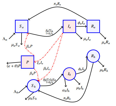
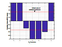
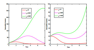
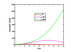
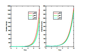
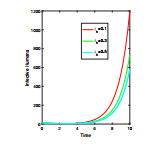
Anthrax is an acute infectious zonootic disease caused by Bacillus anthracis, a gram-positive, rod-shaped non-motile bacterium. It is a disease that mainly affects herbivorous animals of both domestic and wildlife, and causes devastating spillover infections into the human population. Anthrax epidemic results in serious and fatal infections in both animals and humans globally. In this paper, a non-linear differential equation model is proposed to study the transmission dynamics of anthrax in both animal and human populations taking into accounts saturation effect within the animal population and behavioural change of the general public towards the outbreak of the disease. The model is shown to have two unique equilibrium points, namely; the anthrax-free and endemic equilibrium points. The anthrax-free equilibrium point is globally asymptotically stable whenever the reproduction number is less than unity $ (\mathcal{R}_{0} < 1) $ and the endemic equilibrium point is locally asymptotically stable whenever $ \mathcal{R}_{0} > 1 $. Sensitivity analysis suggests that the most influential factors on the spread of anthrax are the infection force $ \beta_{a} $, pathogen shedding rate $ \xi_{a} $, recruitment rate $ \Lambda_a $, natural death rate in animals $ \mu_{a} $ and recovery rate in animals $ \phi_{a} $. Numerical simulations demonstrate that the saturation effect and behavioural change of the general public towards the outbreak of the disease increase the size of the susceptible population, reduce the size of the infective population and the pathogen levels in the environment. Findings of this research show that anthrax epidemic can be controlled by reducing the rate of anthrax infection and pathogen shedding rate, while increasing the rate of pathogen decay through proper environmental hygiene as well as increasing treatment to ensure higher recovery rate in infected animals. The results also show that positive behavioural change of the general public through mass awareness interventions can help control the spread of the disease.
Citation: Elijah B. Baloba, Baba Seidu. A mathematical model of anthrax epidemic with behavioural change[J]. Mathematical Modelling and Control, 2022, 2(4): 243-256. doi: 10.3934/mmc.2022023
Anthrax is an acute infectious zonootic disease caused by Bacillus anthracis, a gram-positive, rod-shaped non-motile bacterium. It is a disease that mainly affects herbivorous animals of both domestic and wildlife, and causes devastating spillover infections into the human population. Anthrax epidemic results in serious and fatal infections in both animals and humans globally. In this paper, a non-linear differential equation model is proposed to study the transmission dynamics of anthrax in both animal and human populations taking into accounts saturation effect within the animal population and behavioural change of the general public towards the outbreak of the disease. The model is shown to have two unique equilibrium points, namely; the anthrax-free and endemic equilibrium points. The anthrax-free equilibrium point is globally asymptotically stable whenever the reproduction number is less than unity $ (\mathcal{R}_{0} < 1) $ and the endemic equilibrium point is locally asymptotically stable whenever $ \mathcal{R}_{0} > 1 $. Sensitivity analysis suggests that the most influential factors on the spread of anthrax are the infection force $ \beta_{a} $, pathogen shedding rate $ \xi_{a} $, recruitment rate $ \Lambda_a $, natural death rate in animals $ \mu_{a} $ and recovery rate in animals $ \phi_{a} $. Numerical simulations demonstrate that the saturation effect and behavioural change of the general public towards the outbreak of the disease increase the size of the susceptible population, reduce the size of the infective population and the pathogen levels in the environment. Findings of this research show that anthrax epidemic can be controlled by reducing the rate of anthrax infection and pathogen shedding rate, while increasing the rate of pathogen decay through proper environmental hygiene as well as increasing treatment to ensure higher recovery rate in infected animals. The results also show that positive behavioural change of the general public through mass awareness interventions can help control the spread of the disease.

| [1] |
J. K. Blackburn, K. M. Mcnyset, A. Curtis, M. E. Hugh-Jones, Modeling the geographic distribution of Bacillus anthracis, the causative agent of anthrax disease, for the contiguous United States using Predictive Ecologic Niche Modeling, The American Journal of Tropical Medicine and Hygiene, 77 (2007), 1103–1110. https://doi.org/10.4269/ajtmh.2007.77.1103 doi: 10.4269/ajtmh.2007.77.1103

|
| [2] | World Health Organisation, Emerging infectious diseases and zoonoses, WHO, India, 2014. |
| [3] | B. Ahmed, Y. Sultana, D. S. M. Fatema, K. Ara, N. Begum, S. M. Mostanzid, et al., Anthrax : An emerging zoonotic disease in Bangladesh, Bangladesh Journal of Medical Microbiology, 4 (2010), 46–50. |
| [4] | D. C. Dragon, R. P. Rennie, The ecology of anthrax spores: Tough but not invincible, The Canadian Veterinary Journal, 36 (1995), 295–301. |
| [5] | J. Decker, Deadly diseases and epidemics - Anthrax. (E. I. Alcamo, Ed.). USA : Chelsea House Publishers, 2003. |
| [6] | C. L. Stoltenow, Anthrax, NDSU Extension, USA, 2021. |
| [7] | J. K. Awoonor-Williams, P. A. Apanga, M. Anyawie, T. Abachie, S. Boidoitsiah, J. L. Opare, et al., Anthrax outbreak investigation among humans and animals in Northern Ghana: Case Report, (2016). |
| [8] | National Center for Emerging and Zoontic Infectious Diseases, Guide to understanding anthrax, Center for Disease Control and Prevention, USA, 2016. |
| [9] |
S. V. Shadomy, T. L. Smith, Zoonosis update, anthrax, Journal of the American Veterinary Medical Association, 233 (2008), 63–72. https://doi.org/10.2460/javma.233.1.63 doi: 10.2460/javma.233.1.63
|
| [10] | A. P. Suma, K. P. Suresh, M. R. Gajendragad, B. A. Kavya, Forecasting anthrax in livestock in Karnataka State using remote sensing and climatic variables, International Journal of Science and Research, 6 (2017), 1891–1897. |
| [11] | Food and Agriculture Organisation of the United Nations, Anthrax outbreaks: A warning for improved prevention, control and heightened awareness, Empres Watch, 2016. |
| [12] |
R. Makurumidze, N. T. Gombe, T. Magure, M. Tshimanga, Investigation of an anthrax outbreak in Makoni District, Zimbabwe, BMC Public Health, 298 (2021), 1–10. https://doi.org/10.1186/s12889-021-10275-0 doi: 10.1186/s12889-021-10275-0
|
| [13] |
A. E. Frankel, S. R. Kuo, D. Dostal, L. Watson, N. S. Duesbery, C. P. Cheng, et al., Pathophysiology of anthrax, Frontiers in Bioscience-Landmark, 14 (2009), 4516–4524. https://doi.org/10.2741/3544 doi: 10.2741/3544
|
| [14] |
I. Kracalik, L. Malania, P. Imnadze, J. K. Blackburn, Human anthrax transmission at the urban rural interface, Georgia, The American Journal of Tropical Medicine and Hygiene, 93 (2015), 1156–1159. https://doi.org/10.4269/ajtmh.15-0242 doi: 10.4269/ajtmh.15-0242
|
| [15] |
A. Fasanella, R. Adone, M. Hugh-Jones, Classification and management of animal anthrax outbreaks based on the source of infection, Ann 1st Super Sanita, 50 (2014), 192–195. https://doi.org/10.4415/ANN_14_02_14 doi: 10.4415/ANN_14_02_14
|
| [16] | J. G. Wright, P. C. Quinn, S. Shadomy, N. Messonnier, Use of anthrax vaccine in the United States recommendations of the Advisory Committee on Immunization Practices(ACIP), MMWR Recomm Rep, 59 (2009). |
| [17] | A. D. Sweeney, W. C. Hicks, X. Cui, Y. Li, Q. P. Eichacker, Anthrax infection, concise clinical review, American Journal of Respiratory and Critical Care Medicine, 184 (2011), 1333–1341. |
| [18] | World Health Organisation, Anthrax in humans and animals (4th ed.). (P. Turnbull, Ed.). WHO Press, 2008. |
| [19] | Fact Sheet, Bacillus anthracis (Anthrax), UPMC Center for Health Security, (2014), 1–4. Available from: www.UPMCHealth Security.org |
| [20] |
H. W. Hethcote, The Mathematics of infectious diseases, SIAM Rev., 42 (2000), 599–653. https://doi.org/10.1137/S0036144500371907 doi: 10.1137/S0036144500371907
|
| [21] |
B. D. Hahn, P. R. Furniss, A deterministic model of an anthrax epizootic: Threshold Results, Ecol. Model., 20 (1983), 233–241. https://doi.org/10.1016/0304-3800(83)90009-1 doi: 10.1016/0304-3800(83)90009-1
|
| [22] |
S. Mushayabasa, Global stability of an anthrax model with environmental decontamination and time delay, Discrete Dynamics in Nature and Society, 2015 (2015). https://doi.org/10.1155/2015/573146 doi: 10.1155/2015/573146
|
| [23] |
A. Friedman, A. Yakubu, Anthrax epizootic and migration: Persistence or extinction, Math. Biosci, 241 (2012), 137–144. https://doi.org/10.1016/j.mbs.2012.10.004 doi: 10.1016/j.mbs.2012.10.004
|
| [24] | Z. M. Sinkie, N. S. Murthy, Modeling and simulation study of anthrax attack on environment, Journal of Multidisciplinary Engineering Science and Technology, 3 (2016), 4574–4578. |
| [25] | S. Osman, O. D. Makinde, M. D. Theuri, Mathematical modelling of the transmission dynamics of anthrax in human and animal population, Mathematical Theory and Modeling, 8 (2018), 47–67. |
| [26] | R. Kumar, C. C. Chow, J. D. Bartels, G. Clermont, A mathematical simulation of the inflammatory response to anthrax infection, Shock Society, 29 (2008), 104–111. |
| [27] |
A. Kashkynbayev, F. A. Rihan, Dynamics of fractional-order epidemic models with general nonlinear incidence rate and time-delay, Mathematics, 9 (2021), 1–17. https://doi.org/10.3390/math9151829 doi: 10.3390/math9151829
|
| [28] | Y. Du, R. Xu, A delayed SIR epidemic model with nonlinear incidence rate and pulse vaccination, J. Appl. Math. Inform., 28 (2010), 1089–1099. |
| [29] |
S. N. Chong, J. M. Tchuenche, R. J. Smith, A mathematical model of avian in uenza with half-saturated incidence, Theory in Biosciences, 133 (2014), 23–38. https://doi.org/10.1007/s12064-013-0183-6 doi: 10.1007/s12064-013-0183-6
|
| [30] |
M. Chinyoka, T. B. Gashirai, S. Mushayabasa, On the dynamics of a fractional-order ebola epidemic model with nonlinear incidence rates, Discrete Dynamics in Nature and Society, 2021 (2021). https://doi.org/10.1155/2021/2125061 doi: 10.1155/2021/2125061
|
| [31] |
L. Han, Z. Ma, H. W. Hethcote, Four predator prey models with infectious diseases, Math. Comput. Model., 34 (2001), 849–858. https://doi.org/10.1016/S0895-7177(01)00104-2 doi: 10.1016/S0895-7177(01)00104-2
|
| [32] | Z. Ma, J. Li, Dynamical modeling and analysis of epidemics, Singapore: World Scientic Publishing Co. Pte. Ltd., 2009. |
| [33] |
V. Capasso, G. Serio, A generalization of the Kermack-Mackendrick deterministic epidemic models, Math. Biosci., 42 (1978), 43–61. https://doi.org/10.1016/0025-5564(78)90006-8 doi: 10.1016/0025-5564(78)90006-8
|
| [34] |
S. Liu, L. Pang, S. Ruan, X. Zhang, Global dynamics of avian influenza epidemic models with psychological effect, Computational and Mathematical Methods in Medicine, 2015 (2015), 913726. https://doi.org/10.1155/2015/913726 doi: 10.1155/2015/913726
|
| [35] |
E. B. Baloba, B. Seidu, C. S. Bornaa, Mathematical analysis of the effects of controls on the transmission dynamics of anthrax in both animal and human populations, Computational and Mathematical Methods in Medicine, 2020 (2020), 1581358. https://doi.org/10.1155/2020/1581358 doi: 10.1155/2020/1581358
|
| [36] | G. Birkhoff, G. Rota, Ordinary differential equations, John Wiley and Sons Inc., New York, 1989. |
| [37] |
P. Van den Driessche, J. Watmough, Reproduction numbers and sub-threshold endemic equilibria for compartmental models of disease transmission, Math. Biosci., 180 (2002), 29–48. https://doi.org/10.1016/S0025-5564(02)00108-6 doi: 10.1016/S0025-5564(02)00108-6
|
| [38] |
C. Castillo-Chavez, B. Song, Dynamical models of tuberculosis and their applications, Math. Biosci. Eng., 1 (2004), 361–404. https://doi.org/10.3934/mbe.2004.1.361 doi: 10.3934/mbe.2004.1.361
|
| [39] | H. R. Thieme, Mathematics in Population Biology, Princeton University Press, 2003. |
| [40] |
C. S. Bornaa, Y. I. Seini, B. Seidu, Modeling zoonotic diseases with treatment in both human and animal populations, Commun. Math. Biol. Neurosci., 2017 (2017). https://doi.org/10.28919/cmbn/3236 doi: 10.28919/cmbn/3236
|
| [41] |
J. K. K. Asamoah, Z. Jin, G. Sun, M. Y. Li, A Deterministic model for Q fever transmission dynamics within dairy cattle herds : Using Sensitivity Analysis and Optimal Controls, Computational and Mathematical Methods in Medicine, 2020 (2020), 6820608. https://doi.org/10.1155/2020/6820608 doi: 10.1155/2020/6820608
|
| [42] |
J. K. K. Asamoah, C. S. Bornaa, B. Seidu, Z. Jin, Mathematical analysis of the effects of controls on transmission dynamics of SARS-CoV-2, Alex. Eng. J., 59 (2020), 5069–5078. https://doi.org/10.1016/j.aej.2020.09.033 doi: 10.1016/j.aej.2020.09.033
|
| [43] |
C. S. Bornaa, B. Seidu, M. I. Daabo, Mathematical analysis of rabies infection, J. Appl. Math., 2020 (2020), 1804270. https://doi.org/10.1155/2020/1804270 doi: 10.1155/2020/1804270
|
| [44] |
B. Seidu, O. D. Makinde, I. Y. Seini, Mathematical analysis of the effects of HIV-Malaria co-infection on workplace productivity, Acta Biotheor., 63 (2015), 151–182. https://doi.org/10.1007/s10441-015-9255-y doi: 10.1007/s10441-015-9255-y
|
| [45] |
B. Seidu, . D. Makinde, I. Y. Seini, Mathematical analysis of an industrial HIV/AID model that incorporates carefree attitude towards sex, Acta Biother., 69 (2021), 257–276. https://doi.org/10.1007/s10441-020-09407-7 doi: 10.1007/s10441-020-09407-7
|
| [46] |
B. Seidu, C. S. Bornaa, O. D. Makinde, An ebola model with hyper-susceptibility, Chaos, Solitons & Fractals, 138 (2020), 109938. https://doi.org/10.1016/j.chaos.2020.109938 doi: 10.1016/j.chaos.2020.109938
|
| [47] |
S. Abagna, B. Seidu, C. S. Bornaa, A mathematical model of the transmission dynamics and control of bovine brucellosis in cattle, Abstr. Appl. Anal., 2022 (2022), 9658567. https://doi.org/10.1155/2022/9658567 doi: 10.1155/2022/9658567
|
| [48] | C. Castillo-Chavez, H. Wenzhang, On the computation $\mathcal{R}_0$ and its role on global stability, IMA J. Appl. Math., 125 (1992), 229–250. |
Figures(11) / Tables(4)
Elijah B. Baloba, Baba Seidu. A mathematical model of anthrax epidemic with behavioural change[J]. Mathematical Modelling and Control, 2022, 2(4): 243-256. doi: 10.3934/mmc.2022023


 DownLoad: