The risk-return relationship is of fundamental significance in the field of economics and finance. It is used to structure investment strategies, allocate resources, as well as assist in the construction of policy and regulatory frameworks. The accurate forecast of the risk-return relationship ensures sound financial decisions, whereas an inaccurate one can underestimate risk and thus lead to losses. The GARCH-M approach is one of the foremost models used in South African literature to investigate the risk-return relationship. This study made a novel and significant contribution, on a local and international level, as it was the first study to investigate GARCH-M type models with different innovation distributions. This study analyzed the JSE ALSI returns of the South African market for the sample period from 05 October 2004 to 05 October 2021. Results revealed that the EGARCH (1, 1)-M with the Skewed Student-t distribution (Skew-t) is optimal relative to the standard GARCH, APARCH and GJR. However, the EGARCH-M Skew-t failed to capture the financial data's asymmetric, volatile and random nature. To improve forecast accuracy, this study applied different nonnormal innovation distributions: the Pearson Type Ⅳ distribution (PIVD), Generalized Extreme Value distribution (GEVD), Generalized Pareto distribution (GPD) and Stable. Model diagnostics revealed that the nonnormal innovation distributions adequately captured asymmetry. The Value at Risk and backtesting procedure found that the PIVD, followed by Stable, outperformed the Extreme Value Theory distributions (GEVD and GPD). Thus, investors, risk managers and policymakers would opt to use the EGARCH-M in combination with the PIVD when modelling the risk-return relationship. The main contribution of this study was to confirm that applying GARCH type models with the conventional and normal type distributions, to a volatile emerging market, is considered ineffective. Therefore, this study recommended the exploration of other innovation distributions, that were not included in the scope of this study, for future research purposes.
Citation: Nitesha Dwarika. The risk-return relationship in South Africa: tail optimization of the GARCH-M approach[J]. Data Science in Finance and Economics, 2022, 2(4): 391-415. doi: 10.3934/DSFE.2022020
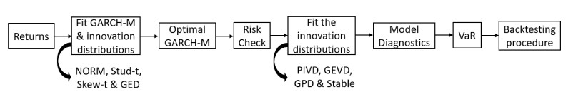
The risk-return relationship is of fundamental significance in the field of economics and finance. It is used to structure investment strategies, allocate resources, as well as assist in the construction of policy and regulatory frameworks. The accurate forecast of the risk-return relationship ensures sound financial decisions, whereas an inaccurate one can underestimate risk and thus lead to losses. The GARCH-M approach is one of the foremost models used in South African literature to investigate the risk-return relationship. This study made a novel and significant contribution, on a local and international level, as it was the first study to investigate GARCH-M type models with different innovation distributions. This study analyzed the JSE ALSI returns of the South African market for the sample period from 05 October 2004 to 05 October 2021. Results revealed that the EGARCH (1, 1)-M with the Skewed Student-t distribution (Skew-t) is optimal relative to the standard GARCH, APARCH and GJR. However, the EGARCH-M Skew-t failed to capture the financial data's asymmetric, volatile and random nature. To improve forecast accuracy, this study applied different nonnormal innovation distributions: the Pearson Type Ⅳ distribution (PIVD), Generalized Extreme Value distribution (GEVD), Generalized Pareto distribution (GPD) and Stable. Model diagnostics revealed that the nonnormal innovation distributions adequately captured asymmetry. The Value at Risk and backtesting procedure found that the PIVD, followed by Stable, outperformed the Extreme Value Theory distributions (GEVD and GPD). Thus, investors, risk managers and policymakers would opt to use the EGARCH-M in combination with the PIVD when modelling the risk-return relationship. The main contribution of this study was to confirm that applying GARCH type models with the conventional and normal type distributions, to a volatile emerging market, is considered ineffective. Therefore, this study recommended the exploration of other innovation distributions, that were not included in the scope of this study, for future research purposes.

| [1] |
Adu G, Alagidede P, Karimu A (2015) Stock return distribution in the BRICKS. Rev Dev Financ 5: 98–109. https://doi.org/10.1016/j.rdf.2015.09.002 doi: 10.1016/j.rdf.2015.09.002

|
| [2] |
Alqaralleh H, Abuhommous AA, Alsaraireh A (2020) Modelling and Forecasting the Volatility of Cryptocurrencies: A Comparison of Nonlinear GARCH-Type Models. Intl J Financ Res 11: 346–356. https://doi.org/10.5430/ijfr.v11n4p346 doi: 10.5430/ijfr.v11n4p346
|
| [3] |
Ayed WB, Fatnassi I, Maatoug AB (2020) Selection of Value-at-Risk models for MENA Islamic indices. J Islamic Account Bus Res 11: 1689–1708. 10.1108/JIABR-07-2019-0122 doi: 10.1108/JIABR-07-2019-0122
|
| [4] |
Bautista RS, Mata LM (2020) A conditional heteroscedastic VaR approach with alternative distributions. EconoQuantum 17: 81–98. https://doi.org/10.18381/eq.v17i2.7125 doi: 10.18381/eq.v17i2.7125
|
| [5] |
Bautista RS, Mora JAN (2020) Value at risk in the oil sector: an analysis of the efficiency in the measurement of the risk of the α-Stable distribution versus the generalized asymmetric Student-t and normal distributions. Contaduría y Administración 65: 1–19. https://doi.org/10.1016/j.physa.2020.124876 doi: 10.1016/j.physa.2020.124876
|
| [6] | Brooks C (2014) Introductory Econometrics for Finance. Cambridge University Press: New York. |
| [7] |
Christoffersen P, Pelletier D (2004) Backtesting Value-at-Risk: A Duration-Based Approach. J Financ Econ 2: 84–108. http://dx.doi.org/10.1093/jjfinec/nbh004 doi: 10.1093/jjfinec/nbh004
|
| [8] |
Christoffersen PF (1998) Evaluating interval forecasts. Int Econ Rev 39: 841–862. https://doi.org/10.2307/2527341 doi: 10.2307/2527341
|
| [9] |
Delis MD, Savva CS, Theodossiou P (2021) The impact of the coronavirus crisis on the market price of risk. J Financ Stab 53(100840): 1–12. https://doi.org/10.1016/j.jfs.2020.100840 doi: 10.1016/j.jfs.2020.100840
|
| [10] |
Ding X, Granger CWJ, Engle, RF (1993) A long memory property of stock market returns and a new model. J Empir Financ 1: 83–106. https://doi.org/10.1016/0927-5398(93)90006-D doi: 10.1016/0927-5398(93)90006-D
|
| [11] |
Dwarika N, Moores-Pitt P, Chifurira R (2021) Volatility dynamics and the risk-return relationship in South Africa: A GARCH approach. Investment Manage Financ Innovations 18: 106–117. http://dx.doi.org/10.21511/imfi.18(2).2021.09 doi: 10.21511/imfi.18(2).2021.09
|
| [12] |
Echaust K, Just M (2020) Value at Risk Estimation Using the GARCH-EVT Approach with Optimal Tail Selection. Math 8: 1–24. http://dx.doi.org/10.3390/math8010114 doi: 10.3390/math8010114
|
| [13] |
Emenogu NG, Adenomon MO, Nweze NO (2020) On the volatility of daily stock returns of Total Nigeria Plc: evidence from GARCH models, value-at-risk and backtesting. Financ Innovation 6: 2–25. https://doi.org/10.1186/s40854-020-00178-1 doi: 10.1186/s40854-020-00178-1
|
| [14] |
Engle RF (1982) Autoregressive Conditional Heteroscedasticity with Estimates of the Variance of United Kingdom Inflation. Econometrica 50: 987–1007. https://doi.org/10.2307/1912773 doi: 10.2307/1912773
|
| [15] |
Engle RF, Lilien D, Robins R (1987) Estimating time varying risk premia in the term structure: the ARCH-M model. Econometrica 55: 391–407. https://doi.org/10.2307/1913242 doi: 10.2307/1913242
|
| [16] |
Glosten LR, Jagannathan R, Runkle DE (1993) On the Relation between the Expected Value and the Volatility of the Nominal Excess Return on Stocks. J Financ 48: 1779–1801. https://doi.org/10.1111/j.1540-6261.1993.tb05128.x doi: 10.1111/j.1540-6261.1993.tb05128.x
|
| [17] | Ilupeju YE (2016) Modelling South Africa's market risk using the APARCH model and heavy-tailed distributions. Master's thesis. University of KwaZulu-Natal. Durban. South Africa. |
| [18] | IRESS (2022) Available from: https://www.iress.com/. |
| [19] | Khan M, Aslam F, Ferreira P (2021) Extreme Value Theory and COVID-19 Pandemic: Evidence from India. Econo Res Guardian 11: 2–10. |
| [20] |
Kuang W (2020) Dynamic VaR forecasts using conditional Pearson type Ⅳ distribution. J Forecasting 2020:1–12. https://doi.org/10.1002/for.2726 doi: 10.1002/for.2726
|
| [21] |
Kupiec PH (1995) Techniques for verifying the accuracy of risk measurement models. J Deriv 3: 73–84. https://doi.org/10.3905/jod.1995.407942 doi: 10.3905/jod.1995.407942
|
| [22] | Ma C, Mi X, Cai Z (2020) Nonlinear and time-varying risk premia. China Econ Rev 62: 1–29. https://doi.org/10.1016/j.chieco.2020.101467 |
| [23] | Mandimika NZ, Chinzara Z (2012) Risk–return trade-off and behaviour of volatility on the South African stock market: evidence from both aggregate and disaggregate data. South African J Econ 80: 345–365. |
| [24] | Mangani R (2008) Modelling return volatility on the JSE Securities Exchange of South Africa. African Financ J 10: 55–71. |
| [25] | Markowitz H (1952) Portfolio selection. J Financ 7: 77–91. |
| [26] |
Naradh K, Chinhamu K, Chifurira R (2021) Estimating the value-at-risk of JSE indices and South African exchange rate with Generalized Pareto and Stable distributions. Investment Manage Financ Innovations 18: 151–165. http://dx.doi.org/10.21511/imfi.18(3).2021.14 doi: 10.21511/imfi.18(3).2021.14
|
| [27] |
Nelson DB (1991) Conditional heteroscedasticity in asset returns: A new approach. Econometrica 59: 347–70. https://doi.org/10.2307/2938260 doi: 10.2307/2938260
|
| [28] |
Omari C, Mundia S, Ngina I (2020) Forecasting Value-at-Risk of Financial Markets under the Global Pandemic of COVID-19 Using Conditional Extreme Value Theory. J Math Financ 10: 569–597. https://doi.org/10.4236/jmf.2020.10403 doi: 10.4236/jmf.2020.10403
|
| [29] |
Saddah S, Sitanggang ML (2020) Value at risk estimation of exchange rate in banking industry. Jurnal Keuangan dan Perbankan 24: 474–484. https://doi.org/10.26905/jkdp.v24i4.4808 doi: 10.26905/jkdp.v24i4.4808
|
| [30] | Tsay RS (2013) An introduction to analysis of financial data with R. Wiley Series in Probability and Statistics. Wiley and Sons. Springer. New Jersey. |


Figures(13) / Tables(14)
Nitesha Dwarika. The risk-return relationship in South Africa: tail optimization of the GARCH-M approach[J]. Data Science in Finance and Economics, 2022, 2(4): 391-415. doi: 10.3934/DSFE.2022020


 DownLoad: