The preparation of moi-moi either from cowpea flour (processed by dry-milling) or paste (processed by wet-milling) has evolved from the indigenous processing methods. Feasibly, freezing should enhance the characteristics of the cowpea grain, and when combined with conventional processing, help to improve emergent products. In this current work, therefore, the combined impact of freezing with soaking times on different cowpea varieties' flour functionality and resultant gel strength, sensory and product yield of moi-moi were studied. Analysis of flour functionality involved the determinations of moisture content, bulk density, oil absorption capacity, swelling index and water absorption capacity, whereas those of moi-moi products involved gel strength, sensory and (product) yield. Across the cowpea flour samples, the functional attributes significantly differed (p < 0.05). Moi-moi products' gel strength of dry-milled appeared higher than wet-milled by specific variety and soaking times. Moi-moi products' sensory attributes of taste, color, texture and general acceptability resembled (p > 0.05), except for the aroma (p < 0.05). Moi-moi products' yield varied widely (p < 0.05) by different reconstituted water volumes. Overall, combining freezing with conventional processing that involved reconstituted water volumes of cowpea promises an enhanced moi-moi yield.
Citation: Ikechukwu O. Amagwula, Chijioke M. Osuji, Gloria C. Omeire, Chinaza G. Awuchi, Charles Odilichukwu R. Okpala. Combined impact of freezing and soaking times on different cowpea varieties' flour functionality and resultant gel strength, sensory and product yield of moi-moi[J]. AIMS Agriculture and Food, 2022, 7(4): 762-776. doi: 10.3934/agrfood.2022047
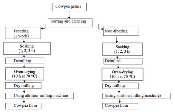
The preparation of moi-moi either from cowpea flour (processed by dry-milling) or paste (processed by wet-milling) has evolved from the indigenous processing methods. Feasibly, freezing should enhance the characteristics of the cowpea grain, and when combined with conventional processing, help to improve emergent products. In this current work, therefore, the combined impact of freezing with soaking times on different cowpea varieties' flour functionality and resultant gel strength, sensory and product yield of moi-moi were studied. Analysis of flour functionality involved the determinations of moisture content, bulk density, oil absorption capacity, swelling index and water absorption capacity, whereas those of moi-moi products involved gel strength, sensory and (product) yield. Across the cowpea flour samples, the functional attributes significantly differed (p < 0.05). Moi-moi products' gel strength of dry-milled appeared higher than wet-milled by specific variety and soaking times. Moi-moi products' sensory attributes of taste, color, texture and general acceptability resembled (p > 0.05), except for the aroma (p < 0.05). Moi-moi products' yield varied widely (p < 0.05) by different reconstituted water volumes. Overall, combining freezing with conventional processing that involved reconstituted water volumes of cowpea promises an enhanced moi-moi yield.

| [1] |
Kebede E, Bekeko Z (2020) Expounding the production and importance of cowpea (Vigna unguiculata (L.) Walp.) in Ethiopia. Cogent Food Agric 6: 1769805. https://doi.org/10.1080/23311932.2020.1769805 doi: 10.1080/23311932.2020.1769805

|
| [2] | Timko MP, Ehlers JD, Roberts PA (2007) Cowpea, In: Kole C (Ed.), Pulses, sugar and tuber crops. Genome mapping and molecular breeding in plants, Berlin, Heidelberg: Springer, 49–67. https://doi.org/10.1007/978-3-540-34516-9_3 |
| [3] | Singh BB (2005) Cowpea[Vigna unguiculata (L.) Walp], In: Singh RJ, Jauhar PP (Eds.), Genetic resources, chromosome engineering and crop improvement, Boca Raton: CRC Press. |
| [4] |
Boukar O, Fatokun CA, Huynh BL, et al. (2016) Genomic tools in cowpea breeding pro-grams: Status and perspectives. Front Plant Sci 7: 757. https://doi.org/10.3389/fpls.2016.00757 doi: 10.3389/fpls.2016.00757
|
| [5] |
Sreerama YN, Sashikala VB, Pratape VM, et al. (2012) Nutrients and antinutrients in cowpea and horse gram flours in comparison to chickpea flour: Evaluation of their flour functionality. Food Chem 131: 462–468. https://doi.org/10.1016/j.foodchem.2011.09.008 doi: 10.1016/j.foodchem.2011.09.008
|
| [6] |
McWatters KH (1990) Functional characteristics of cowpea flours in foods. JAOCS 67: 273–275. https://doi.org/10.1007/BF02539675 doi: 10.1007/BF02539675
|
| [7] |
Vachina MA, Chinnan MS, McWatters KH (2006) Effect of processing variables of cowpea (Vigna unguiculata) meal on the functional properties of cowpea paste and quality of Kara (fried cowpea paste). J Food Quality 29: 552–566. https://doi.org/10.1111/j.1745-4557.2006.00094.x doi: 10.1111/j.1745-4557.2006.00094.x
|
| [8] |
Osuji CM, Nwugo CP, Okoro GI, et al. (2012) Effect of soy flour and maize flour addition on phase separation in moi-moi from soaked cowpea (Vigna unguiculata) and cowpea flour from different cowpea varieties. Nigerian Food J 30: 33–37. https://doi.org/10.1016/S0189-7241(15)30032-1 doi: 10.1016/S0189-7241(15)30032-1
|
| [9] |
Darbour B, Whilson DD, Ofosu DO, et al. (2012) Physical, proximate, functional and pasting properties of flour produced from gamma radiated cowpea (Vigna unguiculata, L. Walp). Radiat Phys Chem 81: 450–457. https://doi.org/10.1016/j.radphyschem.2011.12.015 doi: 10.1016/j.radphyschem.2011.12.015
|
| [10] | Quinn J, Myers R, Cowpea: A Versatile Legume for Hot, Dry Conditions, 2002. Available from: http://www.jeffersoninstitute.org/pdf/cowpea_crop_guide.pdf. |
| [11] |
Machado N, Oppolzer D, Ramos A, et al. (2017) Evaluating the freezing impact on the proximate composition of immature cowpea (Vigna unguiculata L.) pods: Classical versus spectroscopic approaches. J Sci Food Agric 97: 4295–4305. https://doi.org/10.1002/jsfa.8305 doi: 10.1002/jsfa.8305
|
| [12] | Brennan JG, Grandison AS (2012) Food processing handbook, 2 Eds., Weinheim: Wiley-VCH. |
| [13] | Uzuegbu JO, Eke OS (2000) Basic food technology: Principles and practice, Maiden Edition, Owerri: Osprey Publication Centre. |
| [14] |
Frank-Peterside N, Dosumu DO, Njoku HO (2002) Sensory evaluation and proximate analysis of African yam bean (Sphenostylis stenocarpa Harms) moimoi. J Appl Sci Environ Manage 6: 43–48. https://doi.org/10.4314/jasem.v6i2.17175 doi: 10.4314/jasem.v6i2.17175
|
| [15] |
Chandi GK, Sogi DS (2007) Functional properties of rice bran protein concentrates. J Food Eng 79: 592–597. https://doi.org/10.1016/j.jfoodeng.2006.02.018 doi: 10.1016/j.jfoodeng.2006.02.018
|
| [16] | Association of Official Analytical Chemists, Official Methods of Food Analysis, 2010. Available from: www.fao.org/idolrep/006/y6022e/03.htm. |
| [17] |
Kaur S, Singh N, Sodhi NS, et al. (2009) Diversity in properties of seed and flour of kidney bean germplasm. Food Chem 117: 282–289. https://doi.org/10.1016/j.foodchem.2009.04.002 doi: 10.1016/j.foodchem.2009.04.002
|
| [18] |
Kumar V, Fotedar R (2009) Agar extraction process for Gracilaria cliftonii. Carbohyd Polym 78: 813–819. https://doi.org/10.1016/j.carbpol.2009.07.001 doi: 10.1016/j.carbpol.2009.07.001
|
| [19] | Meilgaard MC, Thomas Carr B, Civille GV (1999) Sensory evaluation yechniques, 3 Eds., Boca Raton: CRC Press. https://doi.org/10.1201/9781439832271 |
| [20] |
Çakmakçı S, Topdaş EF, Kalın P, et al. (2015) Antioxidant capacity and functionality of oleaster (Elaeagnus angustifolia L.) flour and crust in a new kind of fruity ice cream. Int J Food Sci Technol 50: 472–481. https://doi.org/10.1111/ijfs.12637 doi: 10.1111/ijfs.12637
|
| [21] |
De Angelis D, Madodé YE, Briffaz A, et al. (2020) Comparing the quality of two traditional fried street foods from the raw material to the end product: The Beninese cowpea-based ata and the Italian wheat-based popizza. Legume Sci 2: e35. https://doi.org/10.1002/leg3.35 doi: 10.1002/leg3.35
|
| [22] |
Oluwole A, Olayinka AF (2011) Effects of dehulling on functional and sensory properties of flours from black beans (Phaseolus vulgaris). J Food Nutr Sci 2: 344–349. https://doi.org/10.4236/fns.2011.24049 doi: 10.4236/fns.2011.24049
|
| [23] | Simpson BK (2012) Food biochemistry and food processing, Ames: John Wiley & Sons. |
| [24] |
Karuna D, Noel G, Dilip K (1996) Production and use of raw potato flour in Mauritian traditional foods. Food Nutr Bull 17: 1–8. https://doi.org/10.1177/156482659601700210 doi: 10.1177/156482659601700210
|
| [25] | Bolade MK (2009) Effect of flour production methods on the yield, physicochemical properties of maize flour and rheological characteristics of a maize-based non fermented food dumpling. Afr J Food Sci 3: 288–298. |
| [26] |
Abu JO, Muller K, Duodu KG, et al. (2005) Functional properties of cowpea (Vigna unguiculata L. Walp) flours and pastes as affected by γ-irradiation. Food Chem 93: 103–111. https://doi.org/10.1016/j.foodchem.2004.09.010 doi: 10.1016/j.foodchem.2004.09.010
|
| [27] | Bourne MC (1981) Food texture and viscosity: Concept and measurement, London: Academic Press. |
| [28] | Kilcast D, Subramaniam P (2011) Food and beverage stability and shelf life, Cambridge: Woodhead Publishing. |
| [29] |
Nyambaka H, Ryley J (2004) Multivariate analysis of the sensory changes in the dehydrated cowpea leaves. Talanta 64: 23–29. https://doi.org/10.1016/j.talanta.2004.02.037 doi: 10.1016/j.talanta.2004.02.037
|
| [30] | Okwunodulu IN, Peter GC, Okwunodulu FU (2019) Proximate quantification and sensory assessment of moi-moi prepared from Bambara nut and cowpea flour blends. Asian Food Sci J 9: 1–11. |


Figures(3) / Tables(5)

Ikechukwu O. Amagwula, Chijioke M. Osuji, Gloria C. Omeire, Chinaza G. Awuchi, Charles Odilichukwu R. Okpala. Combined impact of freezing and soaking times on different cowpea varieties' flour functionality and resultant gel strength, sensory and product yield of moi-moi[J]. AIMS Agriculture and Food, 2022, 7(4): 762-776. doi: 10.3934/agrfood.2022047


 DownLoad: