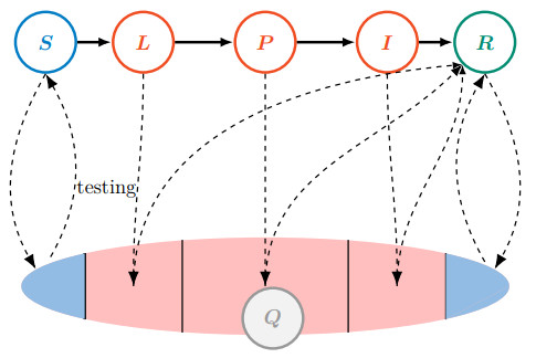
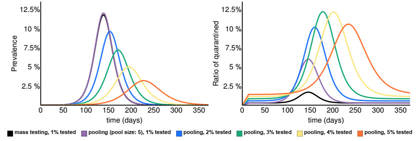
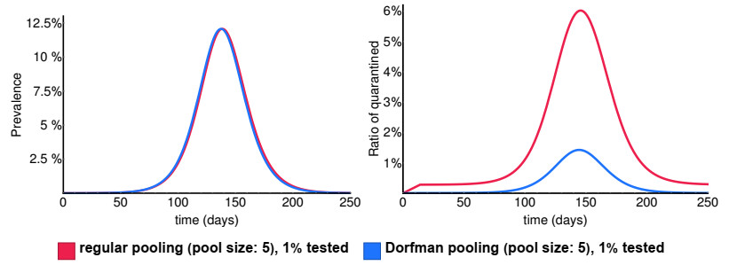
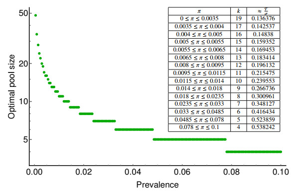
Various measures have been implemented around the world to prevent the spread of SARS-CoV-2. A potential tool to reduce disease transmission is regular mass testing of a high percentage of the population, possibly with pooling (testing a compound of several samples with one single test). We develop a compartmental model to study the applicability of this method and compare different pooling strategies: regular and Dorfman pooling. The model includes isolated compartments as well, from where individuals rejoin the active population after some time delay. We develop a method to optimize Dorfman pooling depending on disease prevalence and establish an adaptive strategy to select variable pool sizes during the course of the epidemic. It is shown that optimizing the pool size can avert a significant number of infections. The adaptive strategy is much more efficient, and may prevent an epidemic outbreak even in situations when a fixed pool size strategy can not.
Citation: Tamás Tekeli, Attila Dénes, Gergely Röst. Adaptive group testing in a compartmental model of COVID-19*[J]. Mathematical Biosciences and Engineering, 2022, 19(11): 11018-11033. doi: 10.3934/mbe.2022513
Various measures have been implemented around the world to prevent the spread of SARS-CoV-2. A potential tool to reduce disease transmission is regular mass testing of a high percentage of the population, possibly with pooling (testing a compound of several samples with one single test). We develop a compartmental model to study the applicability of this method and compare different pooling strategies: regular and Dorfman pooling. The model includes isolated compartments as well, from where individuals rejoin the active population after some time delay. We develop a method to optimize Dorfman pooling depending on disease prevalence and establish an adaptive strategy to select variable pool sizes during the course of the epidemic. It is shown that optimizing the pool size can avert a significant number of infections. The adaptive strategy is much more efficient, and may prevent an epidemic outbreak even in situations when a fixed pool size strategy can not.

| [1] |
P. Boldog, T. Tekeli, Z. Vizi, A. Dénes, F. A. Bartha, G. Röst, Risk assessment of novel coronavirus COVID-19 outbreaks outside China, J. Clin. Med., 9 (2020), 571. https://doi.org/10.3390/jcm9020571 doi: 10.3390/jcm9020571

|
| [2] |
H. Nishiura, S.-M. Jung, N. M. Linton, R. Kinoshita, Y. Yang, K. Hayashi, et al., The extent of transmission of novel coronavirus in Wuhan, China, J. Clin. Med., 9 (2020), 330. https://doi.org/10.3390/jcm9020330 doi: 10.3390/jcm9020330
|
| [3] |
S. Jung, A. R. Akhmetzhanov, K. Hayashi, N. M. Linton, Y. Yang, B. Yuan, et al., Real-time estimation of the risk of death from novel coronavirus (COVID-19) infection: Inference using exported cases, J. Clin. Med., 9 (2020), 523. https://doi.org/10.3390/jcm9020523 doi: 10.3390/jcm9020523
|
| [4] | World Health Organization, Laboratory testing for coronavirus disease (COVID-19) in suspected human cases, Interim guidance, 19 March 2020. https://www.who.int/publications-detail/laboratory-testing-for-2019-novel-coronavirus-in-suspected-human-cases-20200117 |
| [5] | Centers for Disease Control and Prevention, Real-Time RT-PCR Panel for Detection 2019-nCoV, 29 January 2020. https://www.fda.gov/media/134922/download |
| [6] |
P. Habibzadeh, M. Mofatteh, M. Silawi, S. Ghavami, M. A. Faghihi, Molecular diagnostic assays for COVID-19: an overview, Crit. Rev. Clin. Lab. Sci., 58 (2021), 385–398. https://doi.org/10.1080/10408363.2021.1884640 doi: 10.1080/10408363.2021.1884640
|
| [7] |
A. Basu, T. Zinger, K. Inglima, K. Woo, O. Atie, L. Yurasits, et al., Performance of Abbott ID now COVID-19 rapid nucleic acid amplification test using nasopharyngeal swabs transported in viral transport media and dry nasal swabs in a New York City academic institution, J. Clin. Microbiol., 58 (2020), e01136–20. https://doi.org/10.1128/JCM.01136-20 doi: 10.1128/JCM.01136-20
|
| [8] |
B. Berber, C. Aydin, F. Kocabas, G. Guney-Esken, K. Yilancioglu, M. Karadag-Alpaslan, et al., Gene editing and RNAi approaches for COVID-19 diagnostics and therapeutics, Gene Ther., 28 (2021), 290–305. https://doi.org/10.1038/s41434-020-00209-7 doi: 10.1038/s41434-020-00209-7
|
| [9] |
R. W. Peeling, P. L. Olliaro, D. I. Boeras, N. Fongwen, Scaling up COVID-19 rapid antigen tests: promises and challenges, Lancet Infect. Dis., 21 (2021), e290–e295. https://doi.org/10.1016/S1473-3099(21)00048-7 doi: 10.1016/S1473-3099(21)00048-7
|
| [10] | F. A. Bartha, J. Karsai, T. Tekeli, G. Röst, Symptom-based testing in a compartmental model of COVID-19, in Analysis of infectious disease problems (Covid-19) and their global impact (eds. P. Agarwal, J. J. Nieto, M. Ruzhansky, D. F. M. Torres), Springer, Singapore, (2021), 357–376. https://doi.org/10.1007/978-981-16-2450-6_16 |
| [11] |
C. C. Kerr, D. Mistry, R. M. Stuart, K. Rosenfeld, G. R. Hart, R. C. Nunez, et al., Controlling COVID-19 via test-trace-quarantine, Nat. Commun., 12 (2021), 2993. https://doi.org/10.1038/s41467-021-23276-9 doi: 10.1038/s41467-021-23276-9
|
| [12] |
D. Lunz, G. Batt, J. Ruess, To quarantine, or not to quarantine: A theoretical framework for disease control via contact tracing, Epidemics, 34 (2021), 100428. https://doi.org/10.1016/j.epidem.2020.100428 doi: 10.1016/j.epidem.2020.100428
|
| [13] |
J. H. Tanne, E. Hayasaki, M. Zastrow, P. Pulla, P. Smith, A. G. Rada, et al., Covid-19: how doctors and healthcare systems are tackling coronavirus worldwide, BMJ, 368 (2020), m1090. https://doi.org/10.1136/bmj.m1090 doi: 10.1136/bmj.m1090
|
| [14] |
M. Salathé, C. L. Althaus, R. Neher, S. Stringhini, E. Hodcroft, J. Fellay, et al., COVID-19 epidemic in Switzerland: on the importance of testing, contact tracing and isolation, Swiss Med Wkly., 150 (2020), w202205. https://dx.doi.org/10.4414/smw.2020.20225 doi: 10.4414/smw.2020.20225
|
| [15] |
R. Dorfman, The detection of defective members of large populations, Ann. Math. Statistics, 14 (1943), 436–440. https://dx.doi.org/10.1214/aoms/1177731363 doi: 10.1214/aoms/1177731363
|
| [16] |
I. Yelin, N. Aharony, E. Shaer-Tamar, A. Argoetti, E. Messer, D. Berenbaum, et al., Evaluation of COVID-19 RT-qPCR test in multi-sample pools, Clin. Infect. Dis., 71 (2020), 2073–2078. https://dx.doi.org/10.1093/cid/ciaa531 doi: 10.1093/cid/ciaa531
|
| [17] |
Y. Xing, G. W. K. Wong, W. Ni, X. Hu, Q. Xing, Rapid response to an outbreak in Qingdao, China, N. Engl. J. Med., 383 (2020), e129. https://doi.org/10.1056/NEJMc2032361 doi: 10.1056/NEJMc2032361
|
| [18] | Slovakia's mass coronavirus testing finds 57,500 new cases, Financial Times, 10 November 2020. https://www.ft.com/content/6d20007c-25ad-4d1a-b678-591acaa57df9 |
| [19] |
E. Mahase, Operation Moonshot: GP clinics could be used to improve access to COVID-19 tests, BMJ, 370 (2020), m3552. https://doi.org/10.1136/bmj.m3552 doi: 10.1136/bmj.m3552
|
| [20] | Austria to roll out free home coronavirus testing from March, The Local, 15 February 2021. https://www.thelocal.at/20210215/free-coronavirus-home-tests-to-be-rolled-out/ |
| [21] | 'Alles gurgelt', www.allesgurgelt.at. |
| [22] |
R. Verity, L. C. Okell, I. Dorigatti, P. Winskill, C. Whittaker, N. Imai, et al., Estimates of the severity of coronavirus disease 2019: a model-based analysis, Lancet Infect. Dis., 20 (2020), 669–677. https://doi.org/10.1016/S1473-3099(20)30243-7 doi: 10.1016/S1473-3099(20)30243-7
|
| [23] | World Health Organization, Considerations for quarantine of individuals in the context of containment for coronavirus disease (COVID-19), Interim guidance, 19 March 2020. https://apps.who.int/iris/bitstream/handle/10665/331497/WHO-2019-nCoV-IHR_Quarantine-2020.2-eng.pdf |
| [24] |
J. Riou, C. L. Althaus, Pattern of early human-to-human transmission of Wuhan 2019 novel coronavirus (2019-nCoV), December 2019 to January 2020, Euro Surveill., 25 (2020), 2000058. https://doi.org/10.2807/1560-7917.ES.2020.25.4.2000058 doi: 10.2807/1560-7917.ES.2020.25.4.2000058
|
| [25] | R. Moss, J. Wood, D. Brown, F. Shearer, A. J. Black, A. Cheng, et al., Modelling the impact of COVID-19 in Australia to inform transmission reducing measures and health system preparedness, medR$\chi$iv, (2020), 2020.04.07.20056184. https://doi.org/10.1101/2020.04.07.20056184 |
| [26] |
P. Kostoulas, P. Eusebi, S. Hartnack, Diagnostic accuracy estimates for COVID-19 real-time Polymerase Chain Reaction and lateral flow immunoassay tests with bayesian latent-class models, Am. J. Epidemiol., 190 (2021), 1689–1695. https://doi.org/10.1093/aje/kwab093 doi: 10.1093/aje/kwab093
|
| [27] |
S. Clifford, B. J. Quilty, T. W. Russell, Y. Liu, Y-W. D. Chan, C. A. B. Pearson, et al., Strategies to reduce the risk of SARS-CoV-2 re-introduction from international travellers: modelling estimations for the United Kingdom, July 2020. Euro Surveill., 26 (2021), 2001440. https://doi.org/10.2807/1560-7917.ES.2021.26.39.2001440 doi: 10.2807/1560-7917.ES.2021.26.39.2001440
|
| [28] |
J. Hellewell, T. W. Russell, The SAFER Investigators and Field Study Team. et al., Estimating the effectiveness of routine asymptomatic PCR testing at different frequencies for the detection of SARS-CoV-2 infections, BMC Med., 19 (2021), 106. https://doi.org/10.1186/s12916-021-01982-x doi: 10.1186/s12916-021-01982-x
|
| [29] | M. Mancastroppa, R. Burioni, V. Colizza, A. Vezzani, Active and inactive quarantine in epidemic spreading on adaptive activity-driven networks, Phys. Rev. E, 102 2020, 020301(R). https://doi.org/10.1103/PhysRevE.102.020301 |
| [30] | E. Csóka, Application-oriented mathematical algorithms for group testing, arXiv preprint arXiv, (2020), 2005.02388. https://doi.org/10.48550/arXiv.2005.02388 |
Figures(7) / Tables(1)

Tamás Tekeli, Attila Dénes, Gergely Röst. Adaptive group testing in a compartmental model of COVID-19*[J]. Mathematical Biosciences and Engineering, 2022, 19(11): 11018-11033. doi: 10.3934/mbe.2022513


 DownLoad: